Home Page Dirk Bollaerts & Céleste Paalvast

1. Content of exercises of the Jordan normal form

Section 1.
This content section.
Section 2.
We discuss three standard exercises on the Jordan normal form.
Section 3.
We list the matrices that are discussed in the exercises text. This text document can be downloaded, see next 4.
Section 4.
The reader can download the text document in the download section.
Section 5.
The reader can find information about web based material in the information section about links and search material.

2. Jordan normal form: three exercises with solutions

These exercises can be considered standard exercises. For more elaborate explanations, please take a look or download the pdf document provided in the next section.

Exercise 1.

$Jordan structure: (4 \times 4)$ ; $(J_{4} (0))$ .

Use the relevant vector spaces

\ker (B - λ I)^{j}

to investigate and predict the structure of the Jordan normal form of the matrix

B

. Find if possible a matrix

A

similar to

B

such that

A

is a matrix in Jordan normal form. Find explicitly a matrix

P

that is invertible and represents the base change:

A = P^{- 1} B P

Find explicitly Jordan chains that are necessary to construct the matrix $P$ .

B = (\begin{array}{rrrr} 1 & - 2 & 3 & 1 \\ 4 & - 5 & 7 & 2 \\ 3 & - 3 & 4 & 1 \\ - 1 & 0 & 0 & 0 \end{array}) .

Solution.

1. Eigenvalues and the characteristic polynomial.

We check first the eigenvalues by computing the Cayley-Hamilton or characteristic polynomial

p_{C-H} (λ)

p_{C-H} (λ) = | B - λ I_{4} | = λ^{4} .

The eigenvalue

λ = 0

has algebraic multiplicity

4

. The characteristic polynomial

p_{C-H} (λ)

factors completely in linear polynomials over the field

K

. It is thus possible to put the matrix

B

in Jordan normal form over the field

K

2. Digression about a related matrix.

We take a look in this subsection at a related matrix

A

that is already in Jordan normal form. It will later turn out that this is exactly the matrix

A

that we are looking for. A good analysis of this matrix

A

can be a way to better understand what we will do later on in the solution of this exercise starting from the next subsection. Almost every action or calculation we will make from there on has its counterpart here in this subsection in the analysis of the matrix

A

. There will be much less surprises left after this analysis. A more advanced reader can of course skip entirely this subsection and start with subsection 3 of the solution. The solution from that subsection onwards will make no reference at all to this subsection 2. The solution will be completely independent from this section.

We want to investigate the endomorphism

A

associated with this Jordan matrix. We compute also the powers of

A

\begin{aligned} A = (\begin{array}{c} 0 & 1 & 0 & 0 \\ 0 & 0 & 1 & 0 \\ 0 & 0 & 0 & 1 \\ 0 & 0 & 0 & 0 \end{array}), & A^{2} = (\begin{array}{c} 0 & 0 & 1 & 0 \\ 0 & 0 & 0 & 1 \\ 0 & 0 & 0 & 0 \\ 0 & 0 & 0 & 0 \end{array}), \\ A^{3} = (\begin{array}{c} 0 & 0 & 0 & 1 \\ 0 & 0 & 0 & 0 \\ 0 & 0 & 0 & 0 \\ 0 & 0 & 0 & 0 \end{array}), & A^{4} = (\begin{array}{c} 0 & 0 & 0 & 0 \\ 0 & 0 & 0 & 0 \\ 0 & 0 & 0 & 0 \\ 0 & 0 & 0 & 0 \end{array}) . \end{aligned}

We observe that when increasing the exponents of the matrix

A

the original superdiagonals of

1

's in the elementary Jordan blocks of the matrix

A

are going upwards in their respective Jordan blocks in the powers of the matrix

A

until they finally disappear when taking the fourth power of

A

. The matrix itself is already an elementary Jordan block. The smallest exponent that makes the power of the matrix

A

the zero matrix, in this case

4

, is called the height of nilpotency of the matrix

A

It is interesting to observe how the kernels change. We can see almost without calculation that

{\begin{aligned} \ker (A) = span {e_{1}}; \\ \ker (A^{2}) = span {e_{1}, e_{2}}; \\ \ker (A^{3}) = span {e_{1}, e_{2}, e_{3}}; \\ \ker (A^{4}) = span {e_{1}, e_{2}, e_{3}, e_{4}} . \end{aligned}

After having investigated the kernels, we can look at the data we have found in the following information table.

	dim	remaining dim
$\ker (A)$	$1$	$1 = \dim (\ker (A))$
$\ker (A^{2})$	$2$	$1 = \dim (\ker (A^{2})) - \dim (\ker (A))$
$\ker (A^{3})$	$3$	$1 = \dim (\ker (A^{3})) - \dim (\ker (A^{2}))$
$\ker (A^{4})$	$4$	$1 = \dim (\ker (A^{4})) - \dim (\ker (A^{3}))$

We give some explanation about this information table.

We find in the first column the dimensions of the kernels of the consecutive powers of the matrix $A$ .
We have in the second column in every row $i$ but the first the consecutive differences of the kernel dimensions.
In the first row, we have $\dim (\ker (A))$ . This number is equal to the number of elementary Jordan blocks and is usually called the geometric multiplicity of the eigenvalue $λ = 0$ .
The last number of the second column that is not equal to zero, is the number of elementary Jordan chains having the following properties. These elementary Jordan chains consist out of vectors so that their union consists entirely of linearly independent vectors. The lengths of these chains are all exactly equal to the number of the row in which this last non zero number occurs.
The “remaining dim” give the number of linearly independent vectors in Jordan chains that still have to be determined.

We see also that there is equality in the inclusion of sets from the fourth power onwards.

\ker (A) ⊊ \ker (A^{2}) ⊊ \ker (A^{3}) ⊊ \ker (A^{4}) = \ker (A^{5}) = \dots .

This chain of inclusions stabilises from the fourth power onwards.

We mention also the following fact. If

n_{i}

is the number of linearly independent Jordan chains of length exactly

i

, then we have the following set of equations:

{\begin{aligned} n_{1} + n_{2} + n_{3} + n_{4} & = 1 = \dim (\ker (A)), \\ n_{2} + n_{3} + n_{4} & = 1 = \dim (\ker (A^{2})) - \dim (\ker (A)), \\ n_{3} + n_{4} & = 1 = \dim (\ker (A^{3})) - \dim (\ker (A^{2})), \\ n_{4} & = 1 = \dim (\ker (A^{4})) - \dim (\ker (A^{3})) . \end{aligned}

Solving this system, we find

n_{1} = 0

n_{2} = 0

n_{3} = 0

n_{4} = 1

A consequence from this fact is that the numbers in the last column are descending.

We remark by looking at the matrices

A^{i}

that we have the following mappings

{\begin{aligned} A e_{4} = e_{3}, \\ A e_{3} = e_{2}, \\ A e_{2} = e_{1}, \\ A e_{1} = 0, \end{aligned}

{\begin{aligned} A e_{4} = e_{3}, \\ A^{2} e_{4} = e_{2}, \\ A^{3} e_{4} = e_{1}, \\ A^{4} e_{4} = 0 . \end{aligned}

One sees that we have a Jordan chain of linearly independent vectors. We write a Jordan chain in reverse order.

{e_{1} = A^{3} e_{4}, e_{2} = A^{2} e_{4}, e_{3} = A e_{4}, e_{4}} .

After we have found the first Jordan chain of length

4

, we have then the following table.

	dim	chain 1	remaining dim
$ker (A)$	$1$	$e_{1}$	$0$
$ker (A^{2})$	$2$	$e_{2}$	$0$
$ker (A^{3})$	$3$	$e_{3}$	$0$
$ker (A^{4})$	$4$	$e_{4}$	$0$

Because the last column consists now of

0

's, we are done with looking for Jordan chains. We have found at this point a basis of

V

consisting entirely of vectors in Jordan chains.

Let us express our findings in a more visual way that emphasises the dimensions and positions of the elementary Jordan blocks in the matrix.

We give here some comments about the figure.

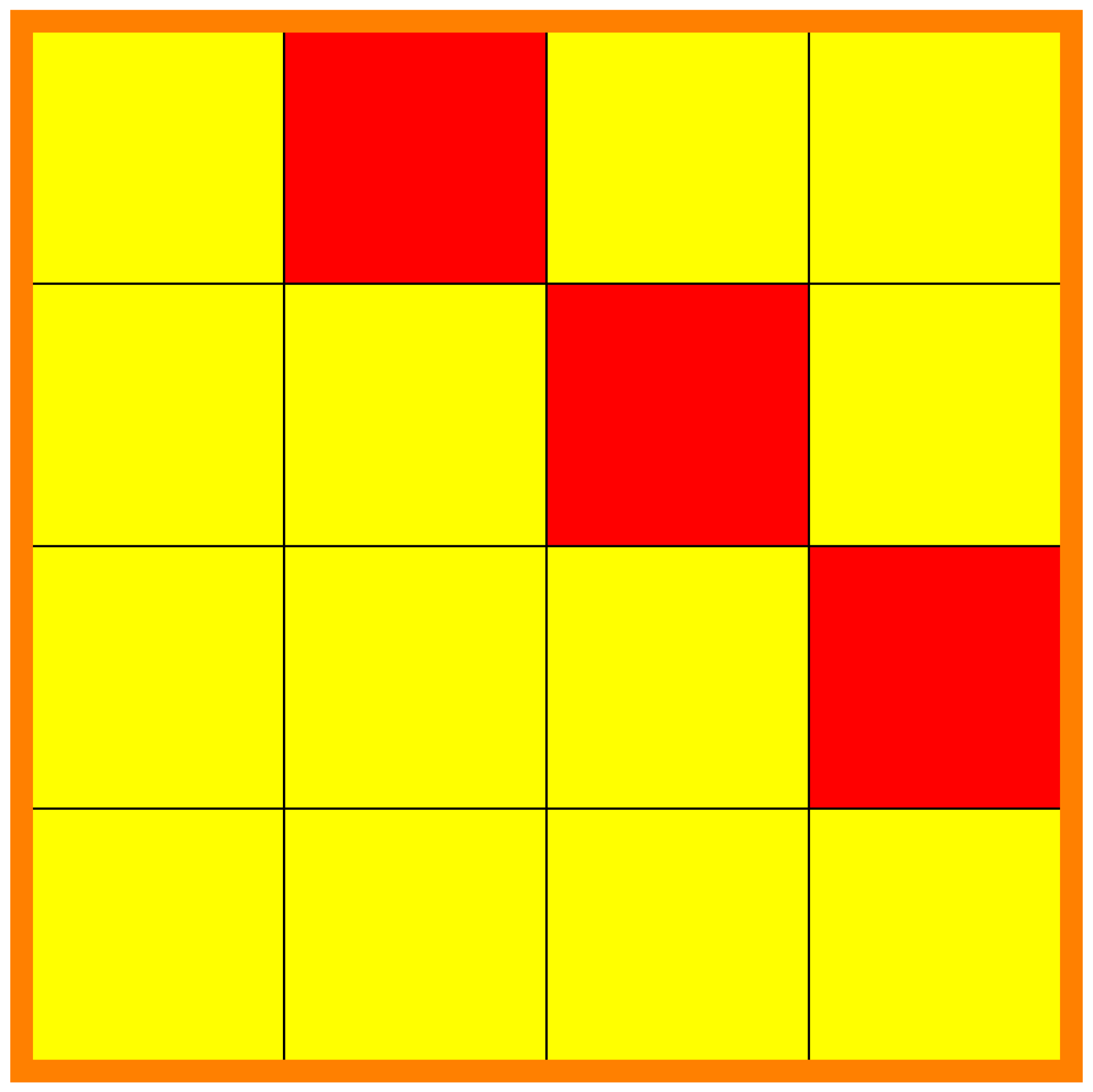
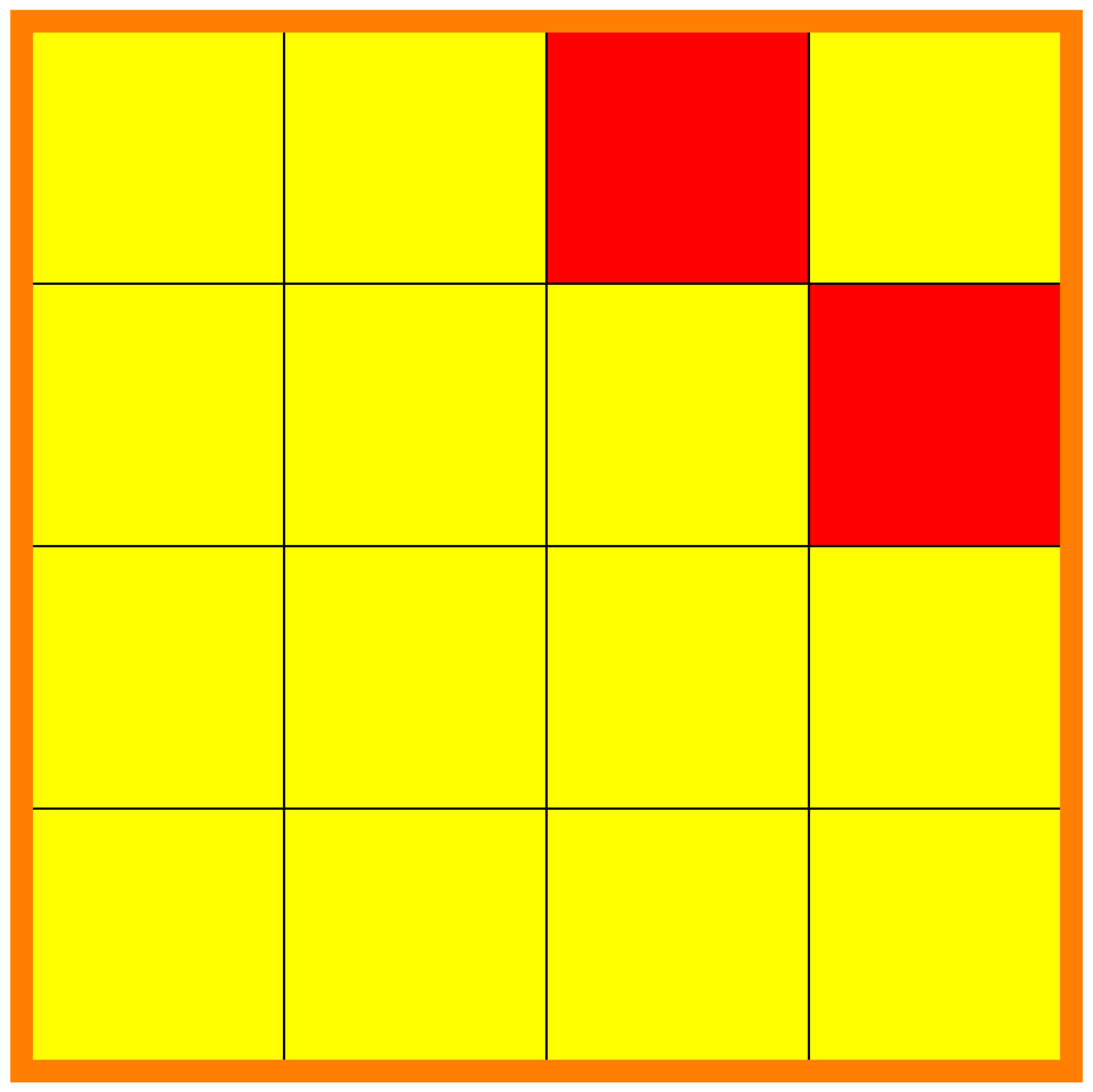
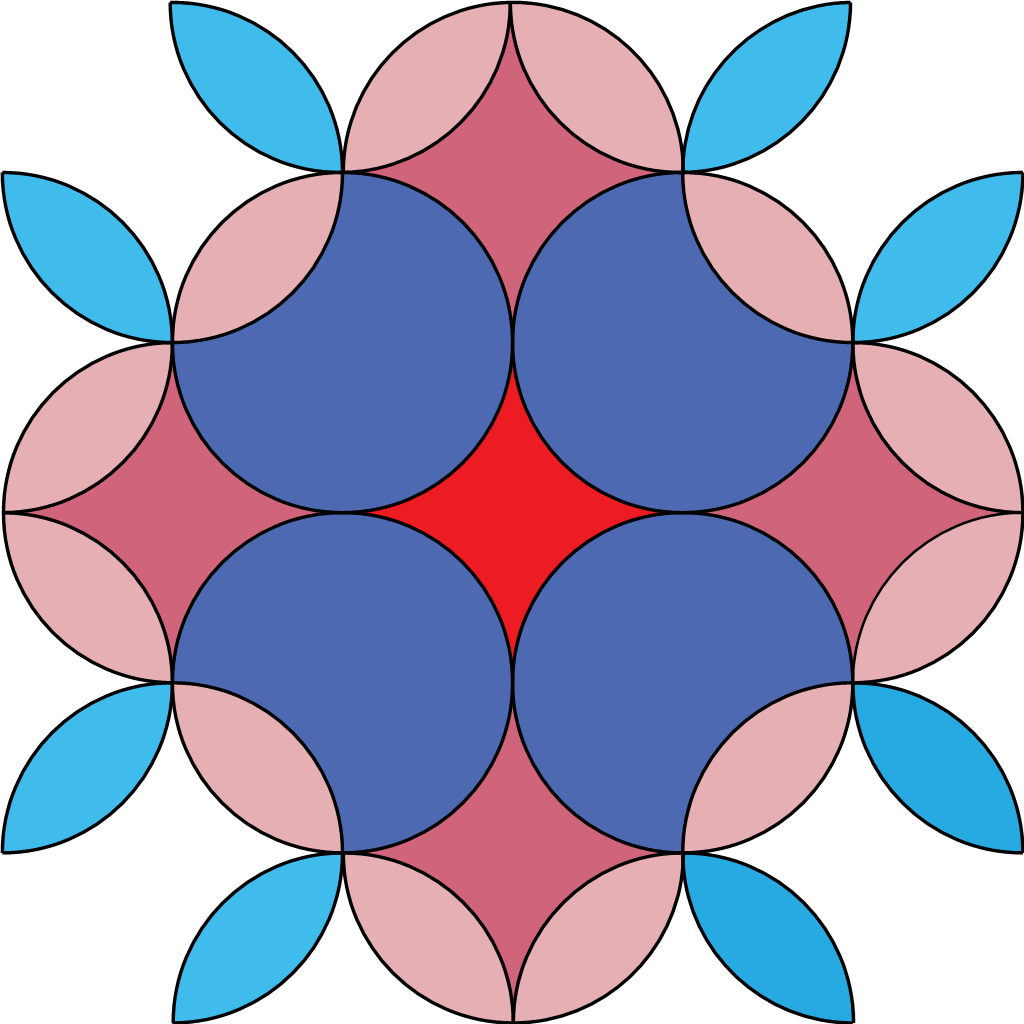
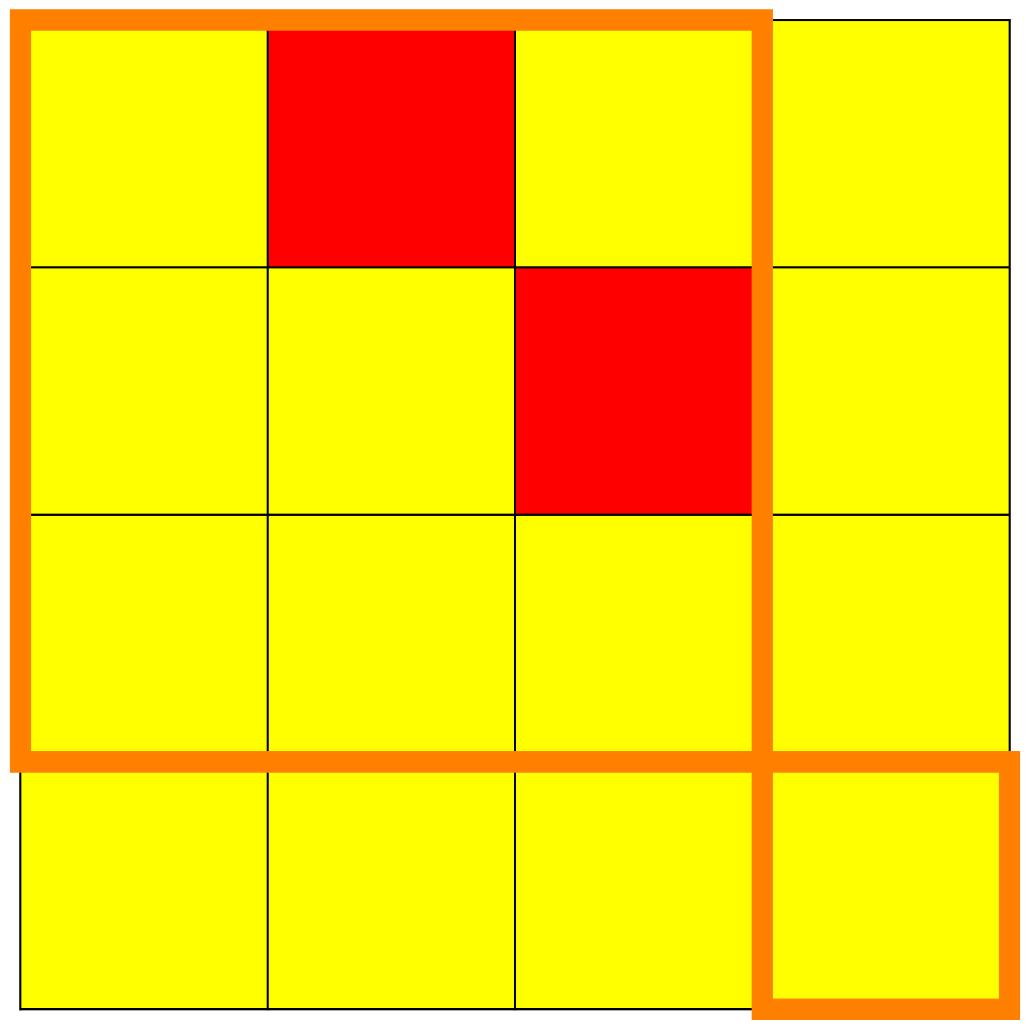
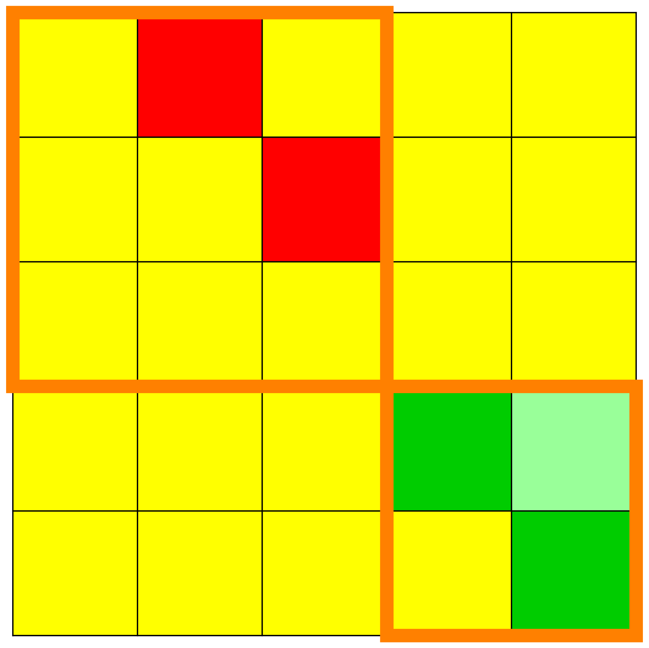
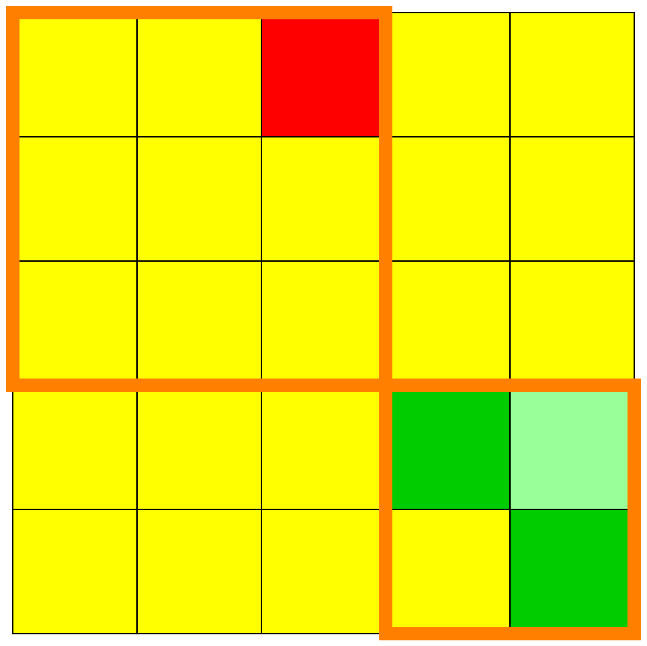
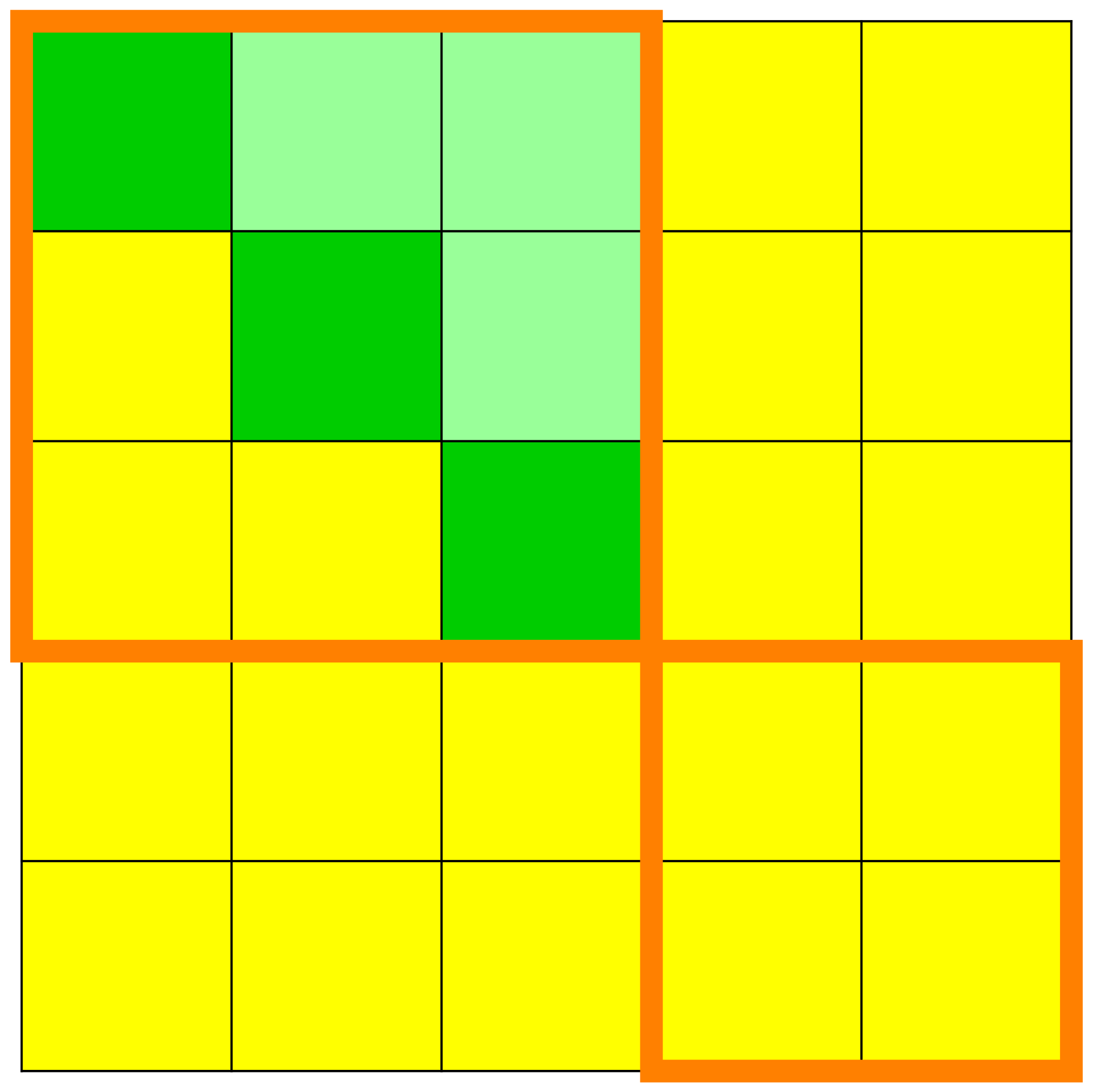
We see in these figures a visualisation of the matrices $A^{i}$ with the squares or cells on which there are $1$ 's, drawn with the colour red, and the squares or cells on which there are $0$ 's, drawn with the colour yellow.
We can immediately observe the kernels of the $A^{i}$ and the dynamic creation of the Jordan chains.
We see also when increasing the exponents how the superdiagonals in the elementary Jordan blocks go steadily higher and higher up into their respective elementary Jordan blocks until they ultimately completely disappear.
We can visually read from these matrices the height of nilpotency.
We can read from these matrices the invariant subspaces with respect to the endomorphism $A$ .
The orange lines delimit the original position of the elementary Jordan blocks.

3. Calculation of the kernels of B^{i} .

Let us calculate the powers of the matrix

B

\begin{aligned} B = (\begin{array}{rrrr} 1 & - 2 & 3 & 1 \\ 4 & - 5 & 7 & 2 \\ 3 & - 3 & 4 & 1 \\ - 1 & 0 & 0 & 0 \end{array}); & B^{2} = (\begin{array}{rrrr} 1 & - 1 & 1 & 0 \\ 3 & - 4 & 5 & 1 \\ 2 & - 3 & 4 & 1 \\ - 1 & 2 & - 3 & - 1 \end{array}); \\ B^{3} = (\begin{array}{rrrr} 0 & 0 & 0 & 0 \\ 1 & - 1 & 1 & 0 \\ 1 & - 1 & 1 & 0 \\ - 1 & 1 & - 1 & 0 \end{array}); & B^{4} = (\begin{array}{cccc} 0 & 0 & 0 & 0 \\ 0 & 0 & 0 & 0 \\ 0 & 0 & 0 & 0 \\ 0 & 0 & 0 & 0 \end{array}) . \end{aligned}

Kernel of B .

We calculate the kernel of

B

and we have to solve the matrix equation

(\begin{array}{rrrr} 1 & - 2 & 3 & 1 \\ 4 & - 5 & 7 & 2 \\ 3 & - 3 & 4 & 1 \\ - 1 & 0 & 0 & 0 \end{array}) (\begin{matrix} z_{1} \\ z_{2} \\ z_{3} \\ z_{4} \end{matrix}) = (\begin{matrix} 0 \\ 0 \\ 0 \\ 0 \end{matrix}) .

This results in the following system of linear equations

{\begin{matrix} z_{1} & - & 2 & z_{2} & + & 3 & z_{3} & + & z_{4} & = & 0, \\ 4 & z_{1} & - & 5 & z_{2} & + & 7 & z_{3} & + & 2 & z_{4} & = & 0, \\ 3 & z_{1} & - & 3 & z_{2} & + & 4 & z_{3} & + & z_{4} & = & 0, \\ - & z_{1} & = & 0. \end{matrix}

This system can be immediately solved and this gives us the solution set or space

\ker (B) = {(0, r_{2}, r_{2}, - r_{2}) ∣ r_{2} \in K} = span {(0, 1, 1, - 1)} .

Kernel of B^{2} .

We calculate the kernel of

B^{2}

and we have to solve the matrix equation

B^{2} = (\begin{array}{rrrr} 1 & - 1 & 1 & 0 \\ 3 & - 4 & 5 & 1 \\ 2 & - 3 & 4 & 1 \\ - 1 & 2 & - 3 & - 1 \end{array}) (\begin{matrix} z_{1} \\ z_{2} \\ z_{3} \\ z_{4} \end{matrix}) = (\begin{matrix} 0 \\ 0 \\ 0 \\ 0 \end{matrix}) .

This results in the following system of linear equations

{\begin{matrix} z_{1} & - & z_{2} & + & z_{3} & = & 0, \\ 3 & z_{1} & - & 4 & z_{2} & + & 5 & z_{3} & + & z_{4} & = & 0, \\ 2 & z_{1} & - & 3 & z_{2} & + & 4 & z_{3} & + & z_{4} & = & 0, \\ - & z_{1} & + & 2 & z_{2} & - & 3 & z_{3} & - & z_{4} & = & 0. \end{matrix}

This system can be immediately solved and this gives us the solution set or space

\begin{aligned} \ker (B^{2}) & = {(r_{1}, r_{2}, - r_{1} + r_{2}, 2 r_{1} - r_{2}) ∣ r_{1}, r_{2} \in K} \\ = span {(1, 0, - 1, 2), (0, 1, 1, - 1)} . \end{aligned}

Kernel of B^{3} .

We calculate the kernel of

B^{3}

and we have to solve the matrix equation

(\begin{array}{rrrr} 0 & 0 & 0 & 0 \\ 1 & - 1 & 1 & 0 \\ 1 & - 1 & 1 & 0 \\ - 1 & 1 & - 1 & 0 \end{array}) (\begin{matrix} z_{1} \\ z_{2} \\ z_{3} \\ z_{4} \end{matrix}) = (\begin{matrix} 0 \\ 0 \\ 0 \\ 0 \end{matrix}) .

This results in the following system of linear equations

{\begin{matrix} z_{1} & - & z_{2} & + & z_{3} & = & 0, \\ z_{1} & - & z_{2} & + & z_{3} & = & 0, \\ - & z_{1} & + & z_{2} & - & z_{3} & = & 0. \end{matrix}

This system can be immediately solved and this gives us the solutions set

\begin{aligned} \ker (B^{3}) & = {(r_{1}, r_{2}, - r_{1} + r_{2}, r_{4}) ∣ r_{1}, r_{2}, r_{4} \in K} \\ = span {(1, 0, - 1, 0), (0, 1, 1, 0), (0, 0, 0, 1)} . \end{aligned}

Kernel of B^{4} .

We want to calculate the kernel of

B^{4}

and we observe first that

B^{4} = (\begin{array}{cccc} 0 & 0 & 0 & 0 \\ 0 & 0 & 0 & 0 \\ 0 & 0 & 0 & 0 \\ 0 & 0 & 0 & 0 \end{array}) .

So the kernel is

K^{4}

We assemble all this information in the following table.

	dim	remaining dim
$\ker (B)$	$1$	$1 = \dim (\ker (B))$
$\ker (B^{2})$	$2$	$1 = \dim (\ker (B^{2})) - \dim (\ker (B))$
$\ker (B^{3})$	$3$	$1 = \dim (\ker (B^{3})) - \dim (\ker (B^{2}))$
$\ker (B^{4})$	$4$	$1 = \dim (\ker (B^{4})) - \dim (\ker (B^{3}))$

We give some explanation about this information table.

We find in the first column the dimensions of the kernels of the consecutive powers of the matrix $B$ .
We have in the second column in every row $i$ but the first the consecutive differences of the kernel dimensions.
In the first row, we have $\dim (\ker (B))$ . This number is equal to the number of elementary Jordan blocks and is usually called the geometric multiplicity of the eigenvalue $λ = 0$ .
The last number of the second column that is not equal to zero, is the number of elementary Jordan chains having the following properties. These elementary Jordan chains consist out of vectors so that their union consists entirely of linearly independent vectors. The lengths of these chains are all exactly equal to the number of the row in which this last non zero number occurs.
The “remaining dim” give the number of linearly independent vectors in Jordan chains that still have to be determined.

The last number in the last column is

1

and this gives the information that there will be a Jordan chain of length

4

. The first number 1 in the last column is the dimension of the kernel of

B

. After we have calculated this chain, the last column will be

{0, 0, 0, 0}

. There are no linearly independent vectors left to be found. We have indeed at that moment already

4

linearly independent vectors which form a base for this vector space.

4. Calculation of the Jordan chains.

The first Jordan chain.

We look for a linearly independent set of vectors

{w_{1}, w_{2}, w_{3}, w_{4}}

satisfying

{\begin{aligned} B w_{1} = 0, \\ B w_{2} = w_{1}, \\ B w_{3} = w_{2}, \\ B w_{4} = w_{3} \end{aligned}

{\begin{aligned} B^{4} w_{4} = 0, \\ B^{3} w_{4} = w_{1}, \\ B^{2} w_{4} = w_{2}, \\ B w_{4} = w_{3} \end{aligned}

where

w_{4}

is in the vector space

\ker (B^{4})

but not in

\ker (B^{3})

We look for a starting

w_{4}

. We see from the information table that there is a generating vector

w_{4}

for a chain of length

4

The generating vector has to satisfy the following conditions.

It has to be in the kernel $\ker (B^{4})$ . So we can describe such a vector as a linear combination of vectors of a basis of the subspace $\ker (B^{4})$ .
The generating vector may not be in the $\ker (B^{3})$ because the length of the chain must be exactly $4$ . So it has to be independent from all vectors in $\ker (B^{3})$ . It is sufficient that it is linearly independent from a basis of $\ker (B^{3})$ .
This generating vector has to be linearly independent from all vectors already chosen in previous Jordan chains which have exactly height $4$ . It can be the case that no previous chains are already chosen or there are no vectors of that height previously chosen in which case this is no condition at all.
We summarise: the generating vector in $B^{4}$ together with the vectors in $\ker (B^{3})$ and also the vectors, if any, of exactly height $4$ chosen in previous Jordan chains must be a linearly independent set of vectors.

Generic form of the generating vector.

We remember that the kernel

\ker (B^{4})

is generated by the following set of vectors.

\begin{aligned} \ker (B^{4}) & = span {e_{1}, e_{2}, e_{3}, e_{4}} . \end{aligned}

So the generating vector has the following generic form

a e_{1} + b e_{2} + c e_{3} + d e_{4} = (a, b, c, d) .

The kernel of B^{3} .

We remember that the kernel

\ker (B^{3})

\ker (B^{3}) = span {(1, 0, - 1, 0), (0, 1, 1, 0), (0, 0, 0, 1)} .

Vectors chosen in previous Jordan chains.

We have previously not chosen any vector in a Jordan chain.

Condition of linear independency of the vectors.

We have to take care that the generic vector is linearly independent of all the vectors mentioned before. We collect for this purpose all these vectors in the rows of the matrix

H

and row reduce then this matrix.

(\begin{array}{cccc} 1 & 0 & - 1 & 0 \\ 0 & 1 & 1 & 0 \\ 0 & 0 & 0 & 1 \\ a & b & c & d \end{array}) .

If we impose the condition

a - b + c \neq 0

, then we can row reduce this matrix to the matrix

(\begin{array}{cccc} 1 & 0 & 0 & 0 \\ 0 & 1 & 0 & 0 \\ 0 & 0 & 1 & 0 \\ 0 & 0 & 0 & 1 \end{array}) .

We conclude that if we impose that

a - b + c \neq 0

, then these vectors are certainly linearly independent.

We can choose

a = 1

b = 0

c = 0

d = 0

and we have the valid generating vector

w_{4} = (1, 0, 0, 0) .

We calculate

B (1, 0, 0, 0)

B^{2} (1, 0, 0, 0)

B^{3} (1, 0, 0, 0)

and we know that the set of vectors

{w_{1} = B^{3} w_{4}, w_{2} = B^{2} w_{4}, w_{3} = B w_{4}, w_{4}}

is a Jordan chain of 4 linearly independent vectors and because

B^{4} w_{4} = 0

we know that the length of the chain is exactly

4

We calculate

w_{3}

w_{3} = B w_{4} = (\begin{array}{rrrr} 1 & - 2 & 3 & 1 \\ 4 & - 5 & 7 & 2 \\ 3 & - 3 & 4 & 1 \\ - 1 & 0 & 0 & 0 \end{array}) (\begin{matrix} 1 \\ 0 \\ 0 \\ 0 \end{matrix}) = (\begin{array}{r} 1 \\ 4 \\ 3 \\ - 1 \end{array})

and

w_{2} = B^{2} w_{4} = (\begin{array}{rrrr} 1 & - 1 & 1 & 0 \\ 3 & - 4 & 5 & 1 \\ 2 & - 3 & 4 & 1 \\ - 1 & 2 & - 3 & - 1 \end{array}) (\begin{matrix} 1 \\ 0 \\ 0 \\ 0 \end{matrix}) = (\begin{array}{r} 1 \\ 3 \\ 2 \\ - 1 \end{array})

and

w_{1} = B^{3} w_{4} = (\begin{array}{rrrr} 0 & 0 & 0 & 0 \\ 1 & - 1 & 1 & 0 \\ 1 & - 1 & 1 & 0 \\ - 1 & 1 & - 1 & 0 \end{array}) (\begin{matrix} 1 \\ 0 \\ 0 \\ 0 \end{matrix}) = (\begin{array}{r} 0 \\ 1 \\ 1 \\ - 1 \end{array}) .

We have now found the Jordan chain

{w_{1} = (0, 1, 1, - 1), w_{2} = (1, 3, 2, - 1), w_{3} = (1, 4, 3, - 1), w_{4} = (1, 0, 0, 0)} .

Let us take a look at our current information table.

	dim	chain 1	remaining dim
$ker (B)$	$1$	$w_{1} = (0, 1, 1, - 1)$	$0$
$ker (B^{2})$	$2$	$w_{2} = (1, 3, 2, - 1)$	$0$
$ker (B^{3})$	$3$	$w_{3} = (1, 4, 3, - 1)$	$0$
$ker (B^{4})$	$4$	$w_{4} = (1, 0, 0, 0)$	$0$

5. Result and check of the result.

We construct the matrix

P

by using the coordinates of the vectors

w_{i}

that we found in the Jordan chains as its columns. We have now

P = (\begin{array}{rrrr} 0 & 1 & 1 & 1 \\ 1 & 3 & 4 & 0 \\ 1 & 2 & 3 & 0 \\ - 1 & - 1 & - 1 & 0 \end{array}) .

\begin{aligned} A = P^{- 1} B P \\ = (\begin{array}{rrrr} 0 & - 1 & 1 & - 1 \\ 0 & 2 & - 3 & - 1 \\ 0 & - 1 & 2 & 1 \\ 1 & - 1 & 1 & 0 \end{array}) (\begin{array}{rrrr} 1 & - 2 & 3 & 1 \\ 4 & - 5 & 7 & 2 \\ 3 & - 3 & 4 & 1 \\ - 1 & 0 & 0 & 0 \end{array}) (\begin{array}{rrrr} 0 & 1 & 1 & 1 \\ 1 & 3 & 4 & 0 \\ 1 & 2 & 3 & 0 \\ - 1 & - 1 & - 1 & 0 \end{array}) \\ = (\begin{array}{cccc} 0 & 1 & 0 & 0 \\ 0 & 0 & 1 & 0 \\ 0 & 0 & 0 & 1 \\ 0 & 0 & 0 & 0 \end{array}) \\ = (\begin{array}{rrrr} 0 & 1 & 0 & 0 \\ 0 & 0 & 1 & 0 \\ 0 & 0 & 0 & 1 \\ 0 & 0 & 0 & 0 \end{array}) . \end{aligned}

Remark that the matrix

A

is itself an elementary Jordan block.

Exercise 2.

$Jordan structure: (4 \times 4)$ ; $(J_{3} (0), J_{1} (0))$ .

Use the relevant vector spaces

\ker (B - λ I)^{j}

to investigate and predict the structure of the Jordan normal form of the matrix

B

. Find if possible a matrix

A

similar to

B

such that

A

is a matrix in Jordan normal form. Find explicitly a matrix

P

that is invertible and represents the base change:

A = P^{- 1} B P

. Find explicitly Jordan chains that are necessary to construct the matrix

P

B = (\begin{array}{rrrr} 1 & 1 & - 2 & 0 \\ 1 & 0 & - 1 & 0 \\ 1 & 0 & - 1 & 0 \\ 0 & 1 & - 1 & 0 \end{array}) .

Solution.

1. Eigenvalues and the characteristic polynomial.

We check first the eigenvalues by computing the Cayley-Hamilton or characteristic polynomial

p_{C-H} (λ)

p_{C-H} (λ) = | B - λ I_{4} | = λ^{4} .

The eigenvalue

λ = 0

has algebraic multiplicity

4

. The characteristic polynomial

p_{C-H} (λ)

factors completely in linear polynomials over the field

K

. It is thus possible to put the matrix

B

in Jordan normal form over the field

K

2. Digression about a related matrix.

We take a look in this subsection at a related matrix

A

that is already in Jordan normal form. It will later turn out that this is exactly the matrix

A

that we are looking for. A good analysis of this matrix

A

A

. There will be much less surprises left after this analysis. A more advanced reader can of course skip entirely this subsection and continue with subsection 3 of the solution. The solution from that subsection onwards will make no reference at all to this subsection 2. The solution will be completely independent from this section.

We will investigate here the matrices

A^{i}

where

A = (\begin{array}{cccc} 0 & 1 & 0 & 0 \\ 0 & 0 & 1 & 0 \\ 0 & 0 & 0 & 0 \\ 0 & 0 & 0 & 0 \end{array}) .

We show the matrix in a coloured way that emphasises the positions of the elementary Jordan blocks.

A = (\begin{array}{rrrr} 0 & 1 & 0 & 0 \\ 0 & 0 & 1 & 0 \\ 0 & 0 & 0 & 0 \\ 0 & 0 & 0 & 0 \end{array}) .

We see that we have a matrix consisting of an elementary Jordan three block and an elementary Jordan one block.

We compute also the powers of

A

\begin{aligned} A = (\begin{array}{c} 0 & 1 & 0 & 0 \\ 0 & 0 & 1 & 0 \\ 0 & 0 & 0 & 0 \\ 0 & 0 & 0 & 0 \end{array}); & A^{2} = (\begin{array}{c} 0 & 0 & 1 & 0 \\ 0 & 0 & 0 & 0 \\ 0 & 0 & 0 & 0 \\ 0 & 0 & 0 & 0 \end{array}); \\ A^{3} = (\begin{array}{c} 0 & 0 & 0 & 0 \\ 0 & 0 & 0 & 0 \\ 0 & 0 & 0 & 0 \\ 0 & 0 & 0 & 0 \end{array}) . \end{aligned}

We observe that when increasing the exponents of the matrix

A

the original superdiagonals of

1

's in the elementary Jordan blocks of the matrix

A

are going upwards in their respective Jordan blocks in the powers of the matrix

A

until they finally disappear when taking the third power of

A

. The smallest exponent that makes the power of the matrix

A

the zero matrix, in this case

3

, is called the height of nilpotency of the matrix

A

It is interesting to observe how the kernels change. We can see almost without calculation that

{\begin{aligned} \ker (A) = span {e_{1}, e_{4}}, \\ \ker (A^{2}) = span {e_{1}, e_{2}, e_{4}}, \\ \ker (A^{3}) = span {e_{1}, e_{2}, e_{3}, e_{4}} . \end{aligned}

After having investigated the kernels, we can look at the data we have found in the following table.

	dim	remaining dim
$\ker (A)$	$2$	$2 = \dim (\ker (A))$
$\ker (A^{2})$	$3$	$1 = \dim (\ker (A^{2})) - \dim (\ker (A))$
$\ker (A^{3})$	$4$	$1 = \dim (\ker (A^{3})) - \dim (\ker (A^{2}))$

We give some explanation about this information table.

We find in the first column the dimensions of the kernels of the consecutive powers of the matrix $A$ .
We have in the second column in every row $i$ but the first the consecutive differences of the kernel dimensions.
In the first row, we have $\dim (\ker (A))$ . This number is equal to the number of elementary Jordan blocks and is usually called the geometric multiplicity of the eigenvalue $λ = 0$ .
The last number of the second column that is not equal to zero, is the number of elementary Jordan chains having the following properties. These elementary Jordan chains consist out of vectors so that their union consists entirely of linearly independent vectors. The lengths of these chains are all exactly equal to the number of the row in which this last non zero number occurs.
The “remaining dim” give the number of linearly independent vectors in Jordan chains that still have to be determined.

We see also that there is equality in the inclusion of sets from the third power onwards.

\ker (A) ⊊ \ker (A^{2}) ⊊ \ker (A^{3}) = \ker (A^{4}) = \dots .

The dimensions of the kernels increase until they stabilise.

We mention also the following fact. If

n_{i}

is the number of linearly independent Jordan chains of length exactly

i

, then we have the following set of equations:

{\begin{aligned} n_{1} + n_{2} + n_{3} & = 2 = \dim (\ker (A)), \\ n_{2} + n_{3} & = 1 = \dim (\ker (A^{2})) - \dim (\ker (A)), \\ n_{3} & = 1 = \dim (\ker (A^{3})) - \dim (\ker (A^{2})) . \end{aligned}

Solving this system, we have

n_{1} = 1

n_{2} = 0

n_{3} = 1

A consequence from this fact is that the numbers in the last column are descending.

We remark by looking at the matrices

A^{i}

that the vector

e_{3}

satisfies

{\begin{aligned} A e_{3} & = e_{2}, \\ A e_{2} & = e_{1}, \\ A e_{1} & = 0 \end{aligned}

{\begin{aligned} A e_{3} = e_{2}, \\ A^{2} e_{3} = e_{1}, \\ A^{3} e_{3} = 0 . \end{aligned}

One sees that we have a Jordan chain of three linearly independent vectors. We write a Jordan chain in reverse order.

{e_{1} = A^{2} e_{3}, e_{2} = A e_{3}, e_{3}} .

After we have found the first Jordan chain of length

3

, we have then the following table.

	dim	chain 1	remaining dim
$ker (A)$	$2$	$e_{1}$	$1$
$ker (A^{2})$	$3$	$e_{2}$	$0$
$ker (A^{3})$	$4$	$e_{3}$	$0$

We look at the last column and see now that we have a second Jordan chain. It has length 1. We have the chain

{e_{4}} .

We have now the following table

	dim	chain 1	chain 2	remaining dim
$ker (A)$	$2$	$e_{1}$	$e_{4}$	$0$
$ker (A^{2})$	$3$	$e_{2}$		$0$
$ker (A^{3})$	$4$	$e_{3}$		$0$

The last column consists entirely out of 0's and we have found a basis for the vector space consisting of vectors in Jordan chains.

Let us express our findings in a way that emphasises the position of the elementary Jordan blocks and their relation with the powers of the matrix

A

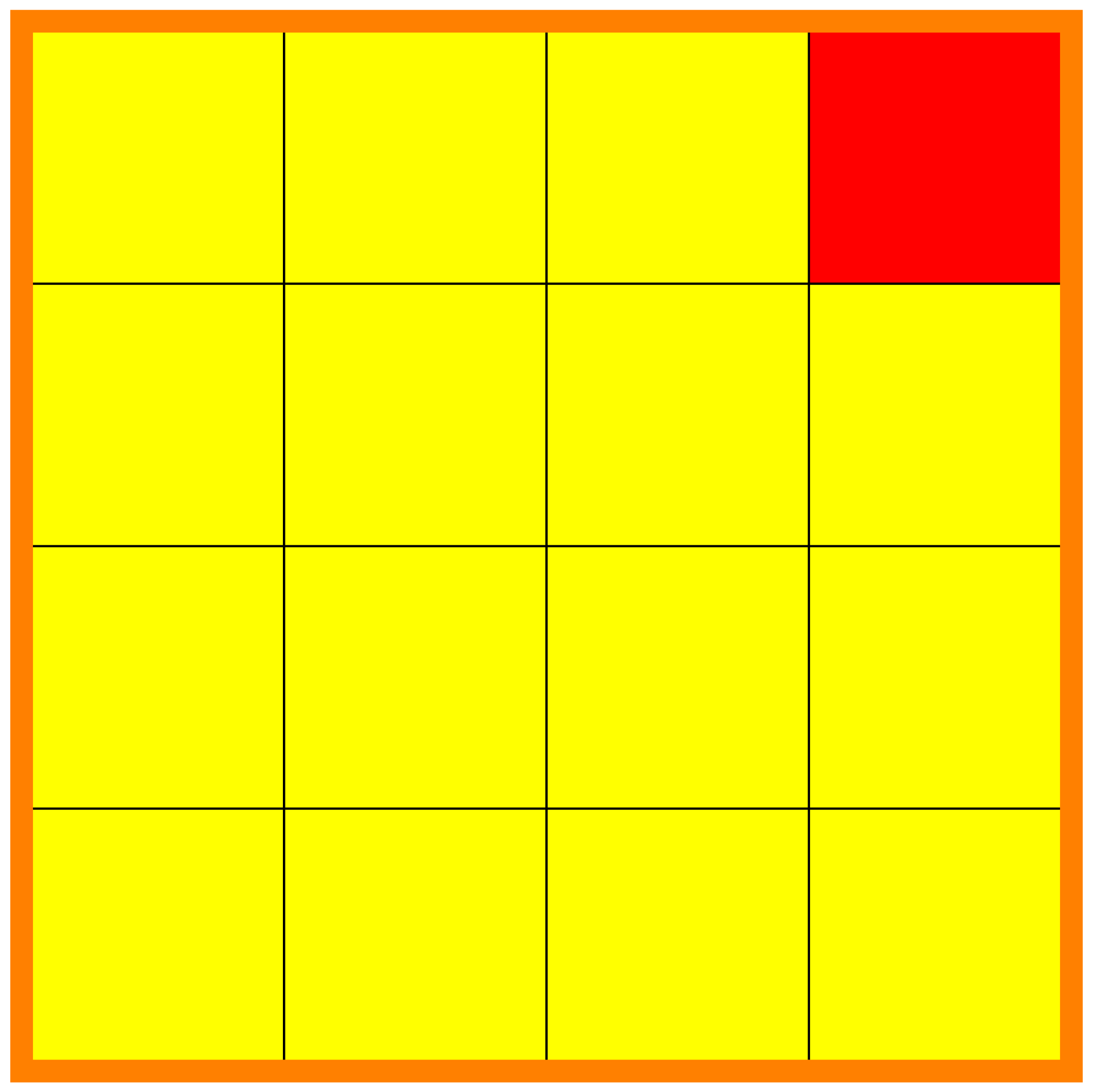
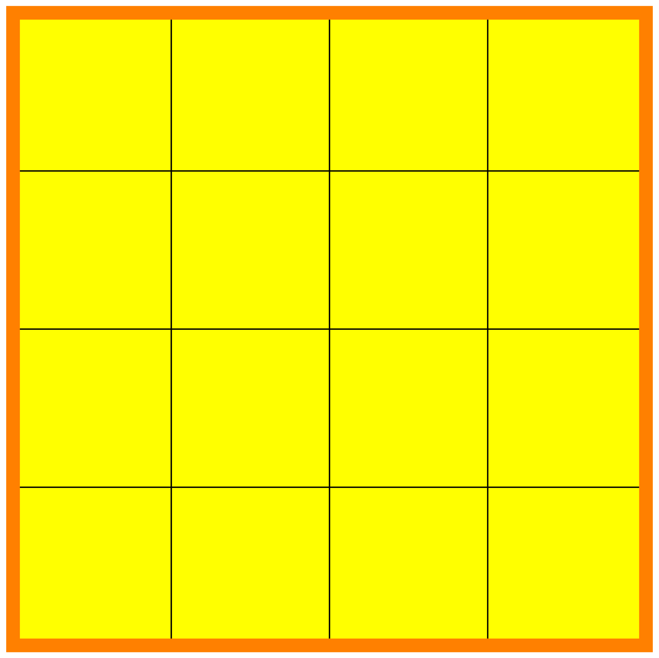
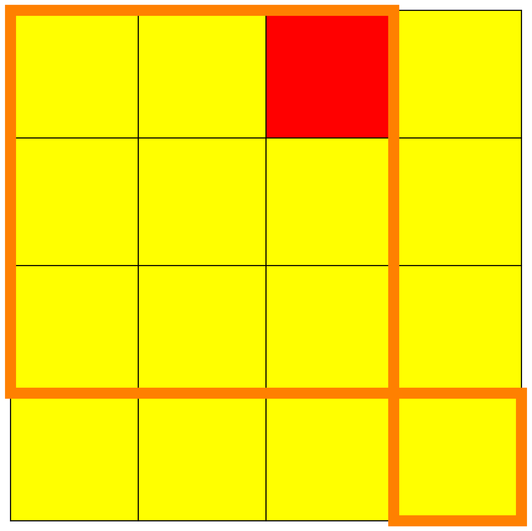
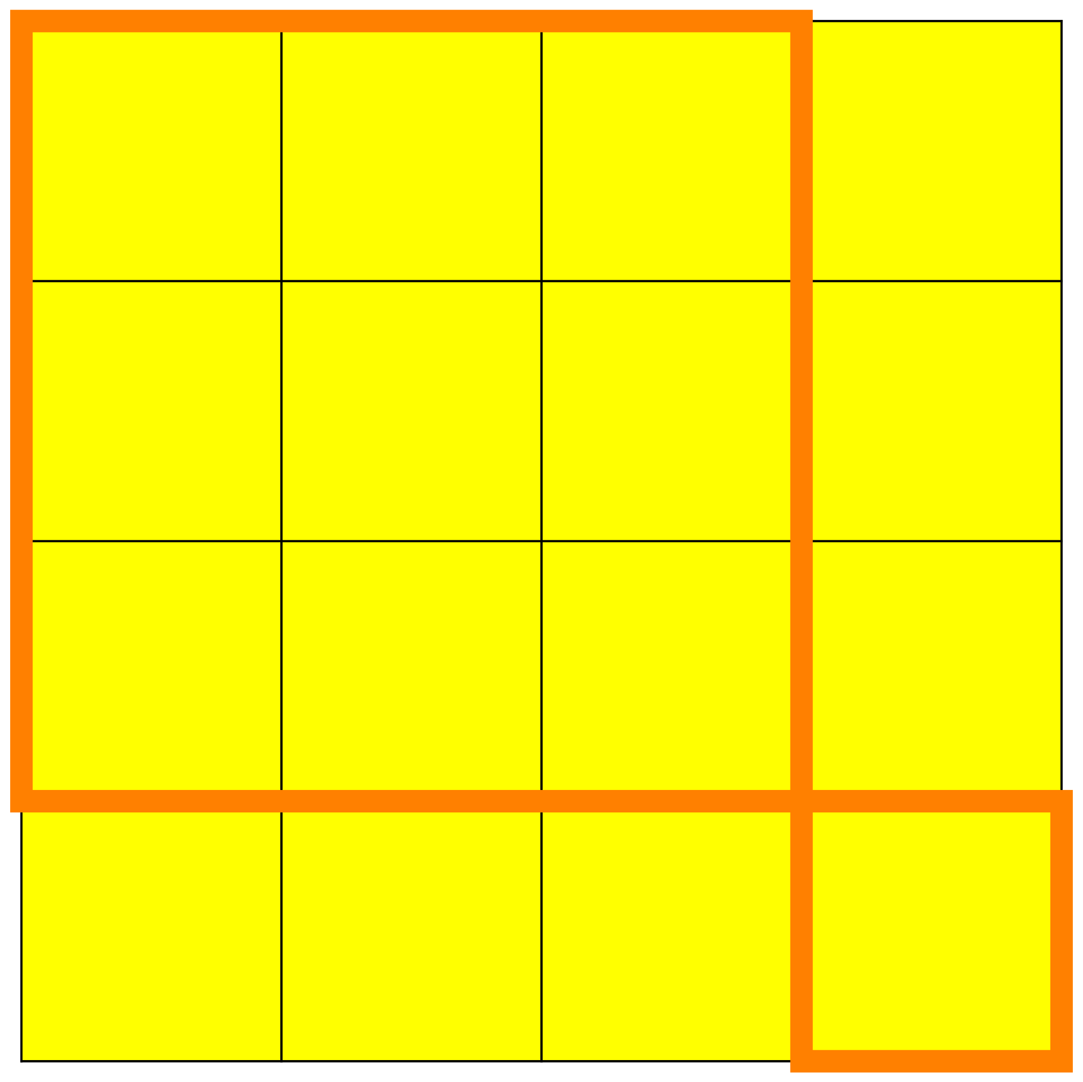
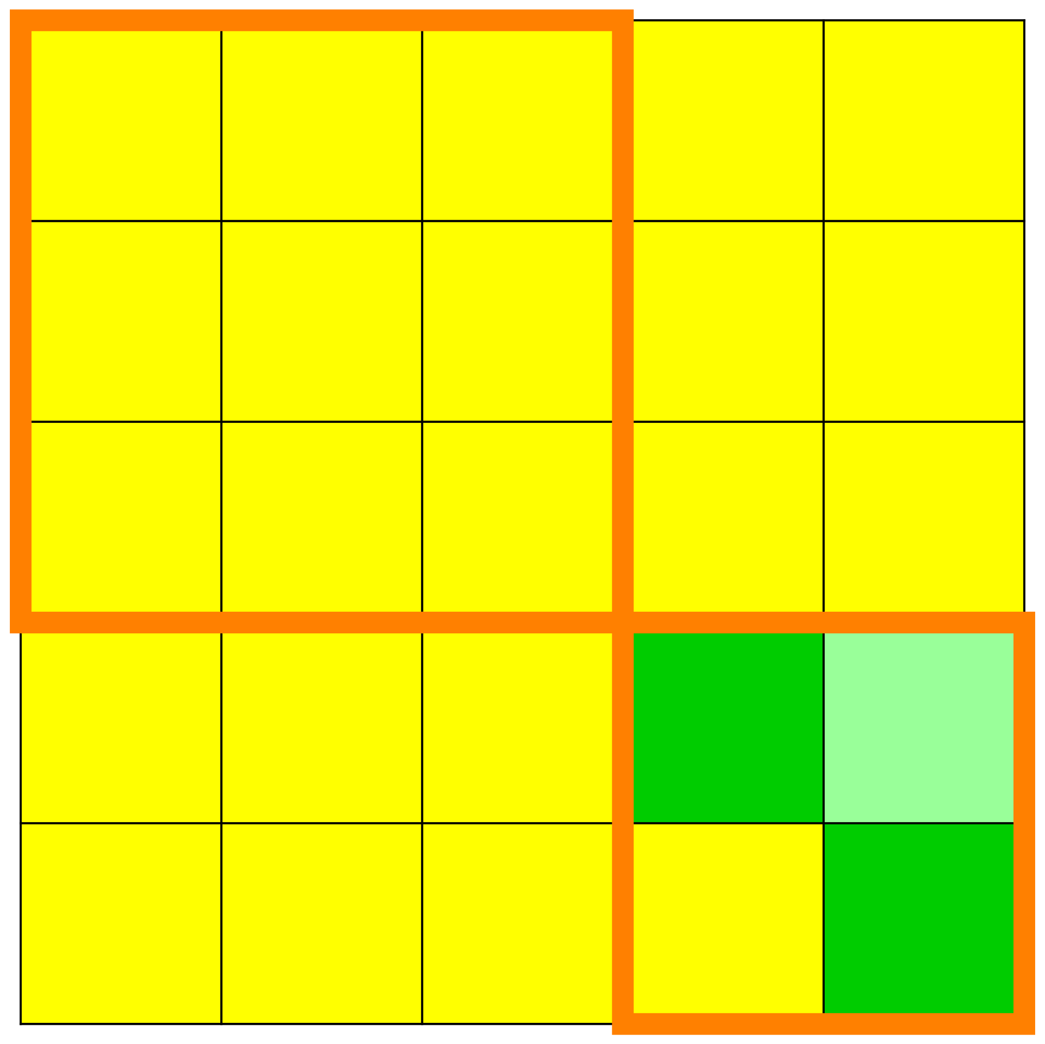
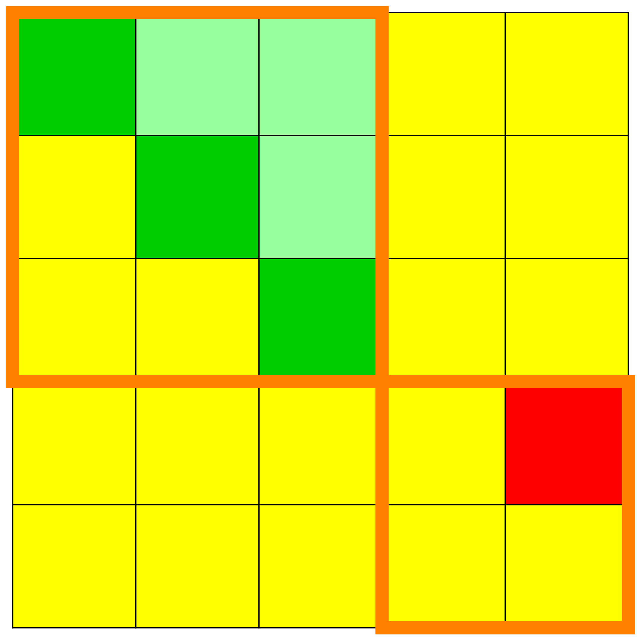
We see in these figures a visualisation of the matrices $A^{i}$ with the squares or cells on which there are $1$ 's, drawn with the colour red, and the squares or cells on which there are $0$ 's, drawn with the colour yellow.
We can immediately observe the kernels of the $A^{i}$ and the dynamic creation of the Jordan chains.
We see also when increasing the exponents how the superdiagonals in the elementary Jordan blocks go steadily higher and higher up into their respective elementary Jordan blocks until they ultimately completely disappear.
We can visually read from these matrices the height of nilpotency.
We can read from these matrices the invariant subspaces with respect to the endomorphism $A$ .
The orange lines delimit the original position of the elementary Jordan blocks.

3. Calculation of the kernels of B^{i} .

\begin{aligned} B = (\begin{matrix} 1 & 1 & - 2 & 0 \\ 1 & 0 & - 1 & 0 \\ 1 & 0 & - 1 & 0 \\ 0 & 1 & - 1 & 0 \end{matrix}); & B^{2} = (\begin{matrix} 0 & 1 & - 1 & 0 \\ 0 & 1 & - 1 & 0 \\ 0 & 1 & - 1 & 0 \\ 0 & 0 & 0 & 0 \end{matrix}); \\ B^{3} = (\begin{matrix} 0 & 0 & 0 & 0 \\ 0 & 0 & 0 & 0 \\ 0 & 0 & 0 & 0 \\ 0 & 0 & 0 & 0 \end{matrix}) . \end{aligned}

Kernel of B .

We calculate the kernel of

B

and we have to solve the matrix equation

(\begin{array}{rrrr} 1 & 1 & - 2 & 0 \\ 1 & 0 & - 1 & 0 \\ 1 & 0 & - 1 & 0 \\ 0 & 1 & - 1 & 0 \end{array}) (\begin{matrix} z_{1} \\ z_{2} \\ z_{3} \\ z_{4} \end{matrix}) = (\begin{matrix} 0 \\ 0 \\ 0 \\ 0 \end{matrix}) .

This results in the following system of linear equations

{\begin{array}{ccccccccccc} z_{1} & + & z_{2} & - & 2 & z_{3} & = & 0, \\ z_{1} & - & z_{3} & = & 0, \\ z_{1} & - & z_{3} & = & 0, \\ z_{2} & - & z_{3} & = & 0. \end{array}

We solve this system and find the solution set which is a subspace

\ker (B) = {(r_{1}, r_{1}, r_{1}, r_{4}) ∣ r_{1}, r_{4} \in K} = span {(1, 1, 1, 0), (0, 0, 0, 1)} .

Kernel of B^{2} .

We calculate the kernel of

B^{2}

and we have to solve the matrix equation

(\begin{array}{rrrr} 0 & 1 & - 1 & 0 \\ 0 & 1 & - 1 & 0 \\ 0 & 1 & - 1 & 0 \\ 0 & 0 & 0 & 0 \end{array}) (\begin{matrix} z_{1} \\ z_{2} \\ z_{3} \\ z_{4} \end{matrix}) = (\begin{matrix} 0 \\ 0 \\ 0 \\ 0 \end{matrix}) .

This results in the following system of linear equations

{\begin{cases} z_{2} & - & z_{3} & = & 0, \\ z_{2} & - & z_{3} & = & 0, \\ z_{2} & - & z_{3} & = & 0. \end{cases}

We solve this system and find the solution set which is a subspace

\begin{aligned} \ker (B^{2}) & = {(r_{1}, r_{2}, r_{2}, r_{4}) ∣ r_{1}, r_{2}, r_{4} \in K} \\ = span {(1, 0, 0, 0), (0, 1, 1, 0), (0, 0, 0, 1)} . \end{aligned}

Kernel of B^{3} .

We calculate the kernel of

B^{3}

and we have to solve the matrix equation

(\begin{array}{rrrr} 0 & 0 & 0 & 0 \\ 0 & 0 & 0 & 0 \\ 0 & 0 & 0 & 0 \\ 0 & 0 & 0 & 0 \end{array}) (\begin{matrix} z_{1} \\ z_{2} \\ z_{3} \\ z_{4} \end{matrix}) = (\begin{matrix} 0 \\ 0 \\ 0 \\ 0 \end{matrix}) .

The solutions set is the space

K^{4}

	dim	remaining dim
$\ker (B)$	$2$	$2 = \dim (\ker (B))$
$\ker (B^{2})$	$3$	$1 = \dim (\ker (B^{2})) - \dim (\ker (B))$
$\ker (B^{3})$	$4$	$1 = \dim (\ker (B^{3})) - \dim (\ker (B^{2}))$

We give some explanation about this information table.

We find in the first column the dimensions of the kernels of the consecutive powers of the matrix $B$ .
We have in the second column in every row $i$ but the first the consecutive differences of the kernel dimensions.
In the first row, we have $\dim (\ker (B))$ . This number is equal to the number of elementary Jordan blocks and is usually called the geometric multiplicity of the eigenvalue $λ = 0$ .
The last number of the second column that is not equal to zero, is the number of elementary Jordan chains having the following properties. These elementary Jordan chains consist out of vectors so that their union consists entirely of linearly independent vectors. The lengths of these chains are all exactly equal to the number of the row in which this last non zero number occurs.
The “remaining dim” give the number of linearly independent vectors in Jordan chains that still have to be determined.

The last number in the last column is

1

and this gives the information that there will be a Jordan chain of length

4

. The first number 1 in the last column is the dimension of the kernel of

B

. After we have calculated this chain, the last column will be

{0, 0, 0, 0}

. There are no linearly independent vectors left to be found. We have indeed at that moment already

4

linearly independent vectors which form a base for this vector space.

4. Calculation of the Jordan chains.

We look for a linearly independent set of vectors

{w_{1}, w_{2}, w_{3}}

satisfying

{\begin{aligned} B w_{1} = 0, \\ B w_{2} = w_{1}, \\ B w_{3} = w_{2} \end{aligned}

{\begin{aligned} B^{3} w_{3} = 0, \\ B^{2} w_{3} = w_{1}, \\ B w_{3} = w_{2} . \end{aligned}

The first Jordan chain.

We look for a generating vector

w_{3}

. We see from the information table that there is a generating vector

w_{3}

for a chain of length

3

The generating vector has to satisfy the following conditions.

It has to be in the kernel $\ker (B^{3})$ . So we can describe such a vector as a linear combination of vectors of a basis of the subspace $\ker (B^{3})$ .
The generating vector may not be in the $\ker (B^{2})$ because the length of the chain must be exactly $3$ . So it has to be independent from all vectors in $\ker (B^{2})$ . It is sufficient that it is linearly independent from a basis of $\ker (B^{2})$ .
This generating vector has to be linearly independent from all vectors already chosen in previous Jordan chains which have exactly height $3$ . It can be the case that no previous chains are already chosen or there are no vectors of that height previously chosen in which case this is no condition at all.
We summarise: the generating vector in $B^{3}$ together with the vectors in $\ker (B^{2})$ and also the vectors, if any, of exactly height $3$ chosen in previous Jordan chains must be a linearly independent set of vectors.

Generic form of the generating vector.

We remember that the kernel

\ker (B^{3})

is generated by the following set of vectors.

\begin{aligned} \ker (B^{3}) & = span {e_{1}, e_{2}, e_{3}, e_{4}} . \end{aligned}

So the generating vector has the following generic form

a e_{1} + b e_{2} + c e_{3} + d e_{4} = (a, b, c, d) .

The kernel of \ker (B^{2}) .

We remember that the kernel

\ker (B^{2})

\ker (B^{2}) = span {(1, 0, 0, 0), (0, 1, 1, 0), (0, 0, 0, 1)} .

Vectors chosen in previous Jordan chains.

We have previously not chosen any vector in a Jordan chain.

Condition of linear independency of the vectors.

We have to take care that the generic vector is linearly independent of all the vectors mentioned before. We collect for this purpose all these vectors in the rows of the matrix

H

and row reduce then this matrix.

H = (\begin{array}{cccc} 1 & 0 & 0 & 0 \\ 0 & 1 & 1 & 0 \\ 0 & 0 & 0 & 1 \\ a & b & c & d \end{array}) .

If we impose the condition

b - c \neq 0

, then we can row reduce this matrix to the matrix

(\begin{array}{cccc} 1 & 0 & 0 & 0 \\ 0 & 1 & 0 & 0 \\ 0 & 0 & 1 & 0 \\ 0 & 0 & 0 & 1 \end{array}) .

We conclude that if we impose that

b - c \neq 0

, then these vectors are certainly linearly independent.

We can choose

a = 0

b = 1

c = 0

and

d = 0

. We have the valid generating vector

w_{3} = (0, 1, 0, 0) .

We calculate

w_{2}

w_{2} = B w_{3} = (\begin{array}{rrrr} 1 & 1 & - 2 & 0 \\ 1 & 0 & - 1 & 0 \\ 1 & 0 & - 1 & 0 \\ 0 & 1 & - 1 & 0 \end{array}) (\begin{matrix} 0 \\ 1 \\ 0 \\ 0 \end{matrix}) = (\begin{array}{r} 1 \\ 0 \\ 0 \\ 1 \end{array})

and

w_{1} = B^{2} w_{3} = (\begin{array}{rrrr} 0 & 1 & - 1 & 0 \\ 0 & 1 & - 1 & 0 \\ 0 & 1 & - 1 & 0 \\ 0 & 0 & 0 & 0 \end{array}) (\begin{matrix} 0 \\ 1 \\ 0 \\ 0 \end{matrix}) = (\begin{array}{r} 1 \\ 1 \\ 1 \\ 0 \end{array}) .

We have found the first Jordan chain.

{w_{1} = (1, 1, 1, 0), w_{2} = (1, 0, 0, 1), w_{3} = (0, 1, 0, 0)} .

Let us take a look at our current information table.

	dim	chain 1	remaining dim
$ker (B)$	$2$	$w_{1}$	$1$
$ker (B^{2})$	$3$	$w_{2}$	$0$
$ker (B^{3})$	$4$	$w_{3}$	$0$

with

w_{1} = (1, 1, 1, 0)

w_{2} = (1, 0, 0, 1)

w_{3} = (0, 1, 0, 0)

We know from the information table that we have one Jordan chain with length

1

left.

The second Jordan chain.

We look for a generating vector

w_{4}

of height 1.

The last column in the information table tells us that there is still a chain of length

1

left to be found. This is an eigenvector

w_{4}

. We know that we have in our previous Jordan chain found an eigenvector

w_{1} = (1, 1, 1, 0)

. So we have to be careful when choosing another eigenvector.

The vector must be an eigenvector. It must be in the space

\ker (B) = span {(1, 1, 1, 0), (0, 0, 0, 1)} .

The vector must be of the generic form

a (1, 1, 1, 0) + b (0, 0, 0, 1) = (a, a, a, b) .

We have at this point chosen in

\ker (B)

already the following vector

w_{1}

of height 1.

w_{1} = (1, 1, 1, 0) .

of height exactly height 1.

We have that the vectors just mentioned must be linearly independent and we place them in the rows of a matrix

H

H = (\begin{array}{cccc} 1 & 1 & 1 & 0 \\ a & a & a & b \end{array}) .

We row reduce this matrix

H

and find then if we impose the condition that

b \neq 0

(\begin{array}{cccc} 1 & 1 & 1 & 0 \\ 0 & 0 & 0 & 1 \end{array}) .

We see that these vectors are independent if we impose the condition

b \neq 0

So we can choose

a = 0

b = 1

We have then generating vector

w_{4} = (0, 0, 0, 1) .

This vector forms a Jordan chain on its own. We have now found the second Jordan chain

{w_{4} = (0, 0, 0, 1)} .

	dim	chain 1	chain 2	remaining dim
$ker (B)$	$2$	$w_{1}$	$w_{4}$	$0$
$ker (B^{2})$	$3$	$w_{2}$		$0$
$ker (B^{3})$	$4$	$w_{3}$		$0$

w_{1} = (1, 1, 1, 0)

w_{2} = (1, 0, 0, 1)

w_{3} = (0, 1, 0, 0)

w_{4} = (0, 0, 0, 1)

The last column tells us that there is nothing left to be found. We have now a basis of vectors consisting of independent Jordan chains.

5. Result and check of the result.

We construct the matrix

P

by using the coordinates of the vectors

w_{i}

that we found in the Jordan chains as its columns. We have now

P = (\begin{array}{rrrr} 1 & 1 & 0 & 0 \\ 1 & 0 & 1 & 0 \\ 1 & 0 & 0 & 0 \\ 0 & 1 & 0 & 1 \end{array}) .

\begin{aligned} A & = P^{- 1} B P \\ = (\begin{array}{rrrr} 0 & 0 & 1 & 0 \\ 1 & 0 & - 1 & 0 \\ 0 & 1 & - 1 & 0 \\ - 1 & 0 & 1 & 1 \end{array}) (\begin{array}{rrrr} 1 & 1 & - 2 & 0 \\ 1 & 0 & - 1 & 0 \\ 1 & 0 & - 1 & 0 \\ 0 & 1 & - 1 & 0 \end{array}) (\begin{array}{rrrr} 1 & 1 & 0 & 0 \\ 1 & 0 & 1 & 0 \\ 1 & 0 & 0 & 0 \\ 0 & 1 & 0 & 1 \end{array}) \\ = (\begin{array}{cccc} 0 & 1 & 0 & 0 \\ 0 & 0 & 1 & 0 \\ 0 & 0 & 0 & 0 \\ 0 & 0 & 0 & 0 \end{array}) \\ = (\begin{array}{rrrr} 0 & 1 & 0 & 0 \\ 0 & 0 & 1 & 0 \\ 0 & 0 & 0 & 0 \\ 0 & 0 & 0 & 0 \end{array}) . \end{aligned}

Exercise 3.

$Jordan structure: (5 \times 5)$ ; $(J_{3} (- 1), J_{2} (2))$ .

Use the relevant vector spaces

\ker (B - λ I)^{j}

to investigate and predict the structure of the Jordan normal form of the matrix

B

. Find if possible a matrix

A

similar to

B

such that

A

is in Jordan normal form. Find explicitly a matrix

P

that is invertible and represents the base change:

A = P^{- 1} B P

. Find explicitly Jordan chains that are necessary to construct the matrix

P

B = (\begin{array}{rrrrr} - 3 & 0 & - 5 & 4 & 1 \\ - 4 & 2 & - 4 & - 1 & - 1 \\ 2 & 1 & 3 & - 5 & 1 \\ 0 & - 1 & 1 & 1 & - 2 \\ 3 & - 2 & 5 & 0 & - 2 \end{array}) .

Solution.

1. Eigenvalues and the characteristic polynomial.

We check first the eigenvalues by computing the Cayley-Hamilton or characteristic polynomial.

p_{C-H} (λ) = | B - λ I_{5} | = - (λ - 2)^{2} (λ + 1)^{3} .

We see that the characteristic Cayley-Hamilton polynomial

p_{C-H} (λ)

can be factorised in linear polynomials over the field

K

. So we can apply the Jordan normalisation machinery.

The eigenvalue

λ = 2

has algebraic multiplicity

2

. The eigenvalue

λ = - 1

has algebraic multiplicity

3

2. Investigation of the first eigenvalue.

We work now with the eigenvalue

λ = - 1

3. Digression about a related matrix.

We take a look in this subsection at a related matrix

A

that is already in Jordan normal form. It will later turn out that this is exactly the matrix

A

that we are looking for. A good analysis of this matrix

A

A

. There will be much less surprises left after this analysis. A more advanced reader can of course skip entirely this subsection and start with subsection 4 of the solution. The solution from that subsection onwards will make no reference at all to this subsection 3. The solution will be completely independent from this section.

We start from the matrix

A

A = (\begin{matrix} - 1 & 1 & 0 & 0 & 0 \\ 0 & - 1 & 1 & 0 & 0 \\ 0 & 0 & - 1 & 0 & 0 \\ 0 & 0 & 0 & 2 & 1 \\ 0 & 0 & 0 & 0 & 2 \end{matrix}) .

We subtract from this matrix

A

the matrix

λ I_{5}

A - λ I_{5} = (\begin{matrix} 0 & 1 & 0 & 0 & 0 \\ 0 & 0 & 1 & 0 & 0 \\ 0 & 0 & 0 & 0 & 0 \\ 0 & 0 & 0 & 3 & 1 \\ 0 & 0 & 0 & 0 & 3 \end{matrix}) .

We compute also the powers of

A - λ I_{5}

A - λ I_{5} = (\begin{matrix} 0 & 1 & 0 & 0 & 0 \\ 0 & 0 & 1 & 0 & 0 \\ 0 & 0 & 0 & 0 & 0 \\ 0 & 0 & 0 & 3 & 1 \\ 0 & 0 & 0 & 0 & 3 \end{matrix}),

(A - λ I_{5})^{2} = (\begin{matrix} 0 & 0 & 1 & 0 & 0 \\ 0 & 0 & 0 & 0 & 0 \\ 0 & 0 & 0 & 0 & 0 \\ 0 & 0 & 0 & 9 & 6 \\ 0 & 0 & 0 & 0 & 9 \end{matrix}),

(A - λ I_{5})^{3} = (\begin{matrix} 0 & 0 & 0 & 0 & 0 \\ 0 & 0 & 0 & 0 & 0 \\ 0 & 0 & 0 & 0 & 0 \\ 0 & 0 & 0 & 27 & 27 \\ 0 & 0 & 0 & 0 & 27 \end{matrix}) .

Let us visualise this situation.

We give here some comment on the preceding figure.

We visualise this type of matrix by colouring the diagonal elements which are not zero by dark green and the colour light green is representing any number. The yellow cells are representing the number zero. The red cells represent the number 1. All the blocks with green cells in it will be keeping the same look however large we take the powers of this matrix.

If we restrict the mapping

A - λ I_{5}

to the subspace

span {e_{1}, e_{2}, e_{3}}

which is an invariant subspace with respect to the operator

A - λ I_{5}

, then we have the classic case of a nilpotent operator on a finite dimensional space. The nilpotent operator has degree of nilpotency

3

. Let us take a look at the first elementary Jordan block in this matrix.

We observe that the original superdiagonal of

1

's in the first block of

A - λ I_{5}

is going upwards in its elementary Jordan block associated with the nilpotent part of the transformation

A - λ I_{5}

when increasing the powers of the matrix

A - λ I_{5}

. It finally disappears when taking the third power of

A - λ I_{5}

Investigation of the first Jordan chain.

It is interesting to observe how the kernels change. We can see almost without calculation that

{\begin{aligned} \ker (A - λ I_{5}) = span {e_{1}}; \\ \ker (A - λ I_{5})^{2} = span {e_{1}, e_{2}}; \\ \ker (A - λ I_{5})^{3} = span {e_{1}, e_{2}, e_{3}} . \end{aligned}

	dim	remaining dim
$\ker (A - λ I_{5})$	$1$	$1 = \dim (\ker (A - λ I_{5}))$
$\ker (A - λ I_{5})^{2}$	$2$	$1 = \dim (\ker (A - λ I_{5})^{2}) - \dim (\ker (A - λ I_{5}))$
$\ker (A - λ I_{5})^{3}$	$3$	$1 = \dim (\ker (A - λ I_{5})^{3}) - \dim (\ker (A - λ I_{5})^{2})$

We find in the first column the dimensions of the kernels. In the second column, we have in every row

i

but the first the consecutive differences of the kernel dimensions numbers

\dim (\ker (A - λ I_{5})^{i}) - \dim (\ker (A - λ I_{5})^{i - 1})

. In the first row, we have

\dim (\ker (A - λ I_{5}))

We see also that there is equality in the inclusion of sets from the third power onwards.

\ker (A - λ I_{5}) ⊊ \ker (A - λ I_{5})^{2} ⊊ \ker (A - λ I_{5})^{3} = \ker (A - λ I_{5})^{4} = \dots .

We remark by looking at the matrices

(A - λ I_{5})^{i}

that we have the following mappings

{\begin{aligned} (A - λ I_{5}) e_{3} = e_{2}, \\ (A - λ I_{5}) e_{2} = e_{1}, \\ (A - λ I_{5}) e_{1} = 0 . \end{aligned}

We remark by looking at the matrices

(A - λ I_{5})^{i}

or as a consequence of the previous mappings that we have also the following mappings

{\begin{aligned} (A - λ I_{5}) e_{3} = e_{2}, \\ (A - λ I_{5})^{2} e_{3} = e_{1}, \\ (A - λ I_{5})^{3} e_{3} = 0 . \end{aligned}

One sees that we have a Jordan chain of linearly independent vectors. We write a Jordan chain in reverse order.

{e_{1} = (A - λ I_{5})^{2} e_{3}, e_{2} = (A - λ I_{5}) e_{3}, e_{3}} .

After we have found the first Jordan chain of length

3

, we have then the following table.

	dim	chain 1	remaining dim
$\ker (A - λ I_{5})$	$1$	$e_{1}$	$0$
$\ker (A - λ I_{5})^{2}$	$2$	$e_{2}$	$0$
$\ker (A - λ I_{5})^{3}$	$3$	$e_{3}$	$0$

We have now in the last column only 0's and this means that we are done looking for Jordan chains.

4. Kernels of (B - λ I_{5})^{i} .

Kernel of (B - λ I_{5}) .

We calculate the kernel of

B - λ I_{5}

The matrix

B - λ I_{5}

B - λ I_{5} = (\begin{matrix} - 2 & 0 & - 5 & 4 & 1 \\ - 4 & 3 & - 4 & - 1 & - 1 \\ 2 & 1 & 4 & - 5 & 1 \\ 0 & - 1 & 1 & 2 & - 2 \\ 3 & - 2 & 5 & 0 & - 1 \end{matrix}) .

We have to solve the matrix equation

(\begin{array}{rrrrr} - 2 & 0 & - 5 & 4 & 1 \\ - 4 & 3 & - 4 & - 1 & - 1 \\ 2 & 1 & 4 & - 5 & 1 \\ 0 & - 1 & 1 & 2 & - 2 \\ 3 & - 2 & 5 & 0 & - 1 \end{array}) (\begin{matrix} z_{1} \\ z_{2} \\ z_{3} \\ z_{4} \\ z_{5} \end{matrix}) = (\begin{matrix} 0 \\ 0 \\ 0 \\ 0 \\ 0 \end{matrix}) .

This results in having to solve the following system of linear equations.

{\begin{cases} - & 2 & z_{1} & - & 5 & z_{3} & + & 4 & z_{4} & + & z_{5} & = & 0, \\ - & 4 & z_{1} & + & 3 & z_{2} & - & 4 & z_{3} & - & z_{4} & - & z_{5} & = & 0, \\ 2 & z_{1} & + & z_{2} & + & 4 & z_{3} & - & 5 & z_{4} & + & z_{5} & = & 0, \\ - & z_{2} & + & z_{3} & + & 2 & z_{4} & - & 2 & z_{5} & = & 0, \\ 3 & z_{1} & - & 2 & z_{2} & + & 5 & z_{3} & - & z_{5} & = & 0. \end{cases}

We solve this system and this gives us the solutions set which is a subspace

\begin{aligned} \ker (B - λ I_{5}) & = {(r_{1}, r_{1} / 2, - r_{1} / 2, 0, - r_{1} / 2) ∣ r_{1} \in K} \\ = span {(1, 1 / 2, - 1 / 2, 0, - 1 / 2)} . \end{aligned}

Kernel of (B - λ I_{5})^{2} .

We calculate the kernel of

(B - λ I_{5})^{2}

The matrix

(B - λ I_{5})^{2}

(B - λ I_{5})^{2} = (\begin{array}{rrrrr} - 3 & - 11 & - 1 & 25 & - 16 \\ - 15 & 8 & - 14 & - 1 & - 8 \\ 3 & 10 & 2 & - 23 & 14 \\ 0 & 0 & 0 & 0 & 0 \\ 9 & 1 & 8 & - 11 & 11 \end{array}) .

We have to solve the matrix equation

(\begin{array}{rrrrr} - 3 & - 11 & - 1 & 25 & - 16 \\ - 15 & 8 & - 14 & - 1 & - 8 \\ 3 & 10 & 2 & - 23 & 14 \\ 0 & 0 & 0 & 0 & 0 \\ 9 & 1 & 8 & - 11 & 11 \end{array}) (\begin{matrix} z_{1} \\ z_{2} \\ z_{3} \\ z_{4} \\ z_{5} \end{matrix}) = (\begin{matrix} 0 \\ 0 \\ 0 \\ 0 \\ 0 \end{matrix}) .

This results in having to solve the following system of linear equations.

{\begin{cases} - & 3 & z_{1} & - & 11 & z_{2} & - & z_{3} & + & 25 & z_{4} & - & 16 & z_{5} & = & 0, \\ - & 15 & z_{1} & + & 8 & z_{2} & - & 14 & z_{3} & - & z_{4} & - & 8 & z_{5} & = & 0, \\ 3 & z_{1} & + & 10 & z_{2} & + & 2 & z_{3} & - & 23 & z_{4} & + & 14 & z_{5} & = & 0, \\ 9 & z_{1} & + & z_{2} & + & 8 & z_{3} & - & 11 & z_{4} & + & 11 & z_{5} & = & 0. \end{cases}

We solve this system and this gives us the solutions set which is a subspace

\begin{aligned} \ker (B - λ I_{5})^{2} & = {(r_{1}, r_{2}, - 2 r_{1} / 3 + r_{2} / 3, - r_{1} / 3 + 2 r_{2} / 3, - 2 r_{1} / 3 + r_{2} / 3) \\ ∣ r_{1}, r_{2} \in K} \\ = span {(1, 0, - 2 / 3, - 1 / 3, - 2 / 3), (0, 1, 1 / 3, 2 / 3, 1 / 3)} . \end{aligned}

Kernel of (B - λ I_{5})^{3} .

We calculate the kernel of

(B - λ I_{5})^{3}

The matrix

(B - λ I_{5})^{3}

(B - λ I_{5})^{3} = (\begin{array}{rrrrr} 0 & - 27 & 0 & 54 & - 27 \\ - 54 & 27 & - 54 & 0 & - 27 \\ 0 & 27 & 0 & - 54 & 27 \\ 0 & 0 & 0 & 0 & 0 \\ 27 & 0 & 27 & - 27 & 27 \end{array}) .

We have to solve the matrix equation

(\begin{array}{rrrrr} 0 & - 27 & 0 & 54 & - 27 \\ - 54 & 27 & - 54 & 0 & - 27 \\ 0 & 27 & 0 & - 54 & 27 \\ 0 & 0 & 0 & 0 & 0 \\ 27 & 0 & 27 & - 27 & 27 \end{array}) (\begin{matrix} z_{1} \\ z_{2} \\ z_{3} \\ z_{4} \\ z_{5} \end{matrix}) = (\begin{matrix} 0 \\ 0 \\ 0 \\ 0 \\ 0 \end{matrix}) .

This results in having to solve the following system of linear equations.

{\begin{array}{rrrrr} - & 54 & z_{1} & + & 27 & z_{2} & - & 54 & z_{3} & - & 27 & z_{5} & = & 0, \\ - & 27 & z_{2} & + & 54 & z_{4} & - & 27 & z_{5} & = & 0, \\ + & 27 & z_{2} & - & 54 & z_{4} & + & 27 & z_{5} & = & 0, \\ 27 & z_{1} & + & 27 & z_{3} & - & 27 & z_{4} & + & 27 & z_{5} & = & 0. \end{array}

We solve this system and this gives us the solutions set which is a subspace

\begin{aligned} \ker (B - λ I_{5})^{3} & = {(r_{1}, r_{2}, r_{3}, - r_{1} + r_{2} - r_{3}, - 2 r_{1} + r_{2} - 2 r_{3}) \\ ∣ r_{1}, r_{2}, r_{3} \in K} \\ = span {(1, 0, 0, - 1, - 2), (0, 1, 0, 1, 1), (0, 0, 1, - 1, - 2)} . \end{aligned}

Kernel of (B - λ I_{5})^{4} .

We calculate the kernel of

(B - λ I_{5})^{4}

The matrix

(B - λ I_{5})^{4}

(B - λ I_{5})^{4} = (\begin{array}{rrrrr} 27 & - 81 & 27 & 135 & - 54 \\ - 189 & 81 & - 189 & 27 & - 108 \\ - 27 & 81 & - 27 & - 135 & 54 \\ 0 & 0 & 0 & 0 & 0 \\ 81 & 0 & 81 & - 81 & 81 \end{array}) .

We have to solve the matrix equation

(\begin{array}{rrrrr} 27 & - 81 & 27 & 135 & - 54 \\ - 189 & 81 & - 189 & 27 & - 108 \\ - 27 & 81 & - 27 & - 135 & 54 \\ 0 & 0 & 0 & 0 & 0 \\ 81 & 0 & 81 & - 81 & 81 \end{array}) (\begin{matrix} z_{1} \\ z_{2} \\ z_{3} \\ z_{4} \\ z_{5} \end{matrix}) = (\begin{matrix} 0 \\ 0 \\ 0 \\ 0 \\ 0 \end{matrix}) .

This results in having to solve the following system of linear equations.

{\begin{matrix} 189 & z_{1} & + & 81 & z_{2} & - & 189 & z_{3} & + & 27 & z_{4} & - & 108 & z_{5} & = & 0, \\ 27 & z_{1} & - & 81 & z_{2} & + & 27 & z_{3} & + & 135 & z_{4} & - & 54 & z_{5} & = & 0, \\ - & 27 & z_{1} & + & 81 & z_{2} & - & 27 & z_{3} & - & 135 & z_{4} & + & 54 & z_{5} & = & 0, \\ 81 & z_{1} & + & 81 & z_{3} & - & 81 & z_{4} & + & 81 & z_{5} & = & 0. \end{matrix}

We solve this system and this gives us the solutions set which is a subspace

\begin{aligned} \ker (B - λ I_{5})^{4} & = {(r_{1}, r_{2}, r_{3}, - r_{1} + r_{2} - r_{3}, - 2 r_{1} + r_{2} - 2 r_{3}) ∣ r_{1}, r_{2}, r_{3} \in K} \\ = span {(1, 0, 0, - 1, - 2), (0, 1, 0, 1, 1), (0, 0, 1, - 1, - 2)} . \end{aligned}

Stabilisation of the kernels.

We see that the kernels are starting to stabilise. We mean by this that we are having equality from the third power onwards in the following chain of inclusion of sets.

\ker (B - λ I_{5}) ⊊ \ker ((B - λ I_{5})^{2}) ⊊ \ker ((B - λ I_{5})^{3}) = \ker ((B - λ I_{5})^{4}) = \dots .

We assemble all this information in the following table.

	dim	remaining dim
$\ker (B - λ I_{5})$	$1$	$1 = \dim (\ker (B - λ I_{5}))$
$\ker (B - λ I_{5})^{2}$	$2$	$1 = \dim (\ker (B - λ I_{5})^{2}) - \dim (\ker (B - λ I_{5}))$
$\ker (B - λ I_{5})^{3}$	$3$	$1 = \dim (\ker (B - λ I_{5})^{3}) - \dim (\ker (B - λ I_{5})^{2})$

The last column in this table is the column of the consecutive differences of the first column,

\dim (\ker ((B - λ I_{5})^{i})) - \dim (\ker ((B - λ I_{5})^{i - 1}))

. The first number of this last column is

\dim (\ker (B - λ I_{5}))

5. Calculation of Jordan chains.

We look for a linearly independent set of vectors

{w_{1}, w_{2}, w_{3}}

satisfying

{\begin{aligned} (B - λ I_{5}) w_{1} = 0, \\ (B - λ I_{5}) w_{2} = w_{1}, \\ (B - λ I_{5}) w_{3} = w_{2} \end{aligned}

{\begin{aligned} (B - λ I_{5})^{3} w_{3} = 0, \\ (B - λ I_{5})^{2} w_{3} = w_{1}, \\ (B - λ I_{5}) w_{3} = w_{2} \end{aligned}

where

w_{3}

is in the vector space

\ker ((B - λ I_{5})^{3})

but not in

\ker ((B - λ I_{5})^{2})

We look for a generating vector

w_{3}

. This vector must be linearly independent of all vectors in

\ker (B - λ I_{5})^{2}

and must be independent from vectors of height 3 that were already chosen in

\ker (B - λ I_{5})^{3}

. We know that

\ker ((B - λ I_{5})^{3}) = span {(1, 0, 0, - 1, - 2), (0, 1, 0, 1, 1), (0, 0, 1, - 1, - 2)} .

We have at this point not chosen any vector of height 3 in

\ker ((B - λ I_{5})^{3})

We know that a vector in

\ker ((B - λ I_{5})^{3})

must be of the form

\begin{aligned} a (1, 0, 0, - 1, - 2) + b (0, 1, 0, 1, 1) + c (0, 0, 1, - 1, - 2) \\ = (a, b, c, - a + b - c, - 2 a + b - 2 c) . \end{aligned}

We remember that

\begin{array}{r} \ker (B - λ I_{5})^{2} = span {(1, 0, - 2 / 3, - 1 / 3, - 2 / 3), (0, 1, 1 / 3, 2 / 3, 1 / 3)} . \end{array}

So we have that the vectors just mentioned must be linearly independent and we place them in the rows of a matrix

H

H = (\begin{array}{ccccc} 1 & 0 & - 2 / 3 & - 1 / 3 & - 2 / 3 \\ 0 & 1 & 1 / 3 & 2 / 3 & 1 / 3 \\ a & b & c & - a + b - c & - 2 a + b - 2 c \end{array}) .

We row reduce this matrix

H

and if we impose

2 a - b + 3 c \neq 0

, we find

(\begin{array}{rrrrr} 1 & 0 & 0 & - 1 & - 2 \\ 0 & 1 & 0 & 1 & 1 \\ 0 & 0 & 1 & - 1 & - 2 \end{array}) .

We see that these vectors are independent if we impose the condition

2 a - b + 3 c \neq 0

. We can choose

a = 1

b = 0

and

c = 0

We have the generating vector

w_{3} = (1, 0, 0, - 1, - 2) .

We start with

w_{3} = (1, 0, 0, - 1, - 2)

We calculate

w_{2}

\begin{aligned} w_{2} & = (B - λ I_{5}) w_{3} \\ = (\begin{array}{rrrrr} - 2 & 0 & - 5 & 4 & 1 \\ - 4 & 3 & - 4 & - 1 & - 1 \\ 2 & 1 & 4 & - 5 & 1 \\ 0 & - 1 & 1 & 2 & - 2 \\ 3 & - 2 & 5 & 0 & - 1 \end{array}) (\begin{array}{r} 1 \\ 0 \\ 0 \\ - 1 \\ - 2 \end{array}) = (\begin{array}{r} - 8 \\ - 1 \\ 5 \\ 2 \\ 5 \end{array}) \end{aligned}

and

\begin{aligned} w_{2} & = (B - λ I_{5})^{2} w_{4} \\ = (\begin{array}{rrrrr} - 3 & - 11 & - 1 & 25 & - 16 \\ - 15 & 8 & - 14 & - 1 & - 8 \\ 3 & 10 & 2 & - 23 & 14 \\ 0 & 0 & 0 & 0 & 0 \\ 9 & 1 & 8 & - 11 & 11 \end{array}) (\begin{array}{r} 1 \\ 0 \\ 0 \\ - 1 \\ - 2 \end{array}) = (\begin{array}{r} 4 \\ 2 \\ - 2 \\ 0 \\ - 2 \end{array}) . \end{aligned}

So we have the Jordan chain

{w_{1} = (4, 2, - 2, 0, - 2), w_{2} = (- 8, - 1, 5, 2, 5), w_{3} = (1, 0, 0, - 1, - 2)} .

Let us take a look at our current information table.

	dim	chain 1	remaining dim
$\ker (B - λ I_{5})$	$1$	$w_{1}$	$0$
$\ker ((B - λ I_{5})^{2})$	$2$	$w_{2}$	$0$
$\ker ((B - λ I_{5})^{3})$	$3$	$w_{3}$	$0$

with

w_{1} = (4, 2, - 2, 0, - 2)

w_{2} = (- 8, - 1, 5, 2, 5)

w_{3} = (1, 0, 0, - 1, - 2)

6. Investigation of the second eigenvalue.

We work now with the eigenvalue

λ = 2

7. Digression about a related matrix.

We take a look in this subsection at a related matrix

A

that is already in Jordan normal form. It will later turn out that this is exactly the matrix

A

that we are looking for. A good analysis of this matrix

A

A

. There will be much less surprises left after this analysis. A more advanced reader can of course skip entirely this subsection and start with subsection 8 of the solution. The solution from that subsection onwards will make no reference at all to this subsection 7. The solution will be completely independent from this section.

We start from the matrix

A

A = (\begin{matrix} - 1 & 1 & 0 & 0 & 0 \\ 0 & - 1 & 1 & 0 & 0 \\ 0 & 0 & - 1 & 0 & 0 \\ 0 & 0 & 0 & 2 & 1 \\ 0 & 0 & 0 & 0 & 2 \end{matrix})

We subtract from this matrix

A

the matrix

λ I_{5}

A - λ I_{5} = (\begin{matrix} - 3 & 1 & 0 & 0 & 0 \\ 0 & - 3 & 1 & 0 & 0 \\ 0 & 0 & - 3 & 0 & 0 \\ 0 & 0 & 0 & 0 & 1 \\ 0 & 0 & 0 & 0 & 0 \end{matrix}) .

We see that the space

span {e_{4}, e_{5}}

is invariant relative to

A - λ I_{5}

. If we restrict

A - λ I_{5}

to this space, we have a nilpotent operator and we can apply the techniques learned in part 2.

We want to investigate the endomorphism

A - λ I_{5}

restricted to this space. We compute now the powers of

A - λ I_{5}

A - λ I_{5} = (\begin{matrix} - 3 & 1 & 0 & 0 & 0 \\ 0 & - 3 & 1 & 0 & 0 \\ 0 & 0 & - 3 & 0 & 0 \\ 0 & 0 & 0 & 0 & 1 \\ 0 & 0 & 0 & 0 & 0 \end{matrix}),

(A - λ I_{5})^{2} = (\begin{matrix} 9 & - 6 & 1 & 0 & 0 \\ 0 & 9 & - 6 & 0 & 0 \\ 0 & 0 & 9 & 0 & 0 \\ 0 & 0 & 0 & 0 & 0 \\ 0 & 0 & 0 & 0 & 0 \end{matrix}) .

Let us visualise this situation.

We give here some comment on the preceding figure.

We visualise this type of matrix by colouring the diagonal elements which are not zero by dark green and the colour light green is representing any number. The yellow cells represent the number 0. The red cells represent the number 1. All the blocks with green cells in it will be keeping the same look however large we take the powers of this matrix.

If we restrict the mapping

A - λ I_{5}

to the subspace

span {e_{4}, e_{5}}

which is an invariant subspace with respect to the operator

A - λ I_{5}

, then we have the classic case of a nilpotent operator on a finite dimensional space. The nilpotent operator has degree of nilpotency

2

. Let us take a look at the second elementary Jordan block in this matrix. We observe that the original superdiagonal of

1

's in the second block of

A - λ I_{5}

are going upwards in their respective elementary Jordan blocks associated with the nilpotent part of the transformation

A - λ I_{5}

when increasing the powers of the matrix

A - λ I_{5}

. It finally disappears when taking the second power of

A - λ I_{5}

All these green elementary Jordan blocks have the same look however large the exponent of

A - λ I_{5}

. The yellow cells are representing the number zero. The nilpotent part of the matrix is the second elementary Jordan block. It changes by moving the superdiagonal upwards when increasing the exponents of

A - λ I_{5}

Investigation of the first Jordan chain.

It is interesting to observe how the kernels change. We can see almost without calculation that

{\begin{aligned} \ker (A - λ I_{5}) = span {e_{4}}; \\ \ker (A - λ I_{5})^{2} = span {e_{4}, e_{5}} . \end{aligned}

	dim	remaining dim
$\ker (A - λ I_{5})^{2}$	$1$	$1 = \dim (\ker (A - λ I_{5}))$
$\ker (A - λ I_{5})^{2}$	$2$	$1 = \dim (\ker (A - λ I_{5})^{2}) - \dim (\ker (A - λ I_{5}))$

We find in the first column the dimensions of the kernels. In the second column, we have in every row

i

but the first the consecutive differences of the kernel dimensions numbers

\dim (\ker (A - λ I_{5})^{i}) - \dim (\ker (A - λ I_{5})^{i - 1})

. In the first row, we have

\dim (\ker (A - λ I_{5}))

We see also that there is equality in the inclusion of sets from the second power onwards.

\ker (A - λ I_{5}) ⊊ \ker (A - λ I_{5})^{2} = \ker (A - λ I_{5})^{3} = \dots .

We remark by looking at the matrices

(A - λ I_{5})^{i}

that we have the following mappings

{\begin{aligned} (A - λ I_{5}) e_{5} = e_{4}, \\ (A - λ I_{5}) e_{4} = 0 . \end{aligned}

We remark by looking at the matrices

(A - λ I_{5})^{i}

or as a consequence of the previous mappings that we have also the following mappings

{\begin{aligned} (A - λ I_{5}) e_{5} = e_{4}, \\ (A - λ I_{5})^{2} e_{5} = 0 . \end{aligned}

One sees that we have a Jordan chain of linearly independent vectors. We write a Jordan chain in reverse order.

{e_{4} = (A - λ I_{5}) e_{5}, e_{5}} .

After we have found the Jordan chain of length

2

, we have then the following table.

	dim	chain 1	remaining dim
$\ker (A - λ I_{5})$	$1$	$e_{4}$	$0$
$\ker (A - λ I_{5})^{2}$	$2$	$e_{5}$	$0$

We have now in the last column only 0's and this means that we are done looking for Jordan chains.

8.
Kernels of (B - λ I_{5})^{i} .

Kernel of (B - λ I_{5}) .

We calculate the kernel of

B - λ I_{5}

The matrix

B - λ I_{5}

B - λ I_{5} = (\begin{array}{rrrrr} - 2 & 0 & - 5 & 4 & 1 \\ - 4 & 3 & - 4 & - 1 & - 1 \\ 2 & 1 & 4 & - 5 & 1 \\ 0 & - 1 & 1 & 2 & - 2 \\ 3 & - 2 & 5 & 0 & - 1 \end{array}) .

We have to solve the matrix equation

(\begin{array}{rrrrr} - 2 & 0 & - 5 & 4 & 1 \\ - 4 & 3 & - 4 & - 1 & - 1 \\ 2 & 1 & 4 & - 5 & 1 \\ 0 & - 1 & 1 & 2 & - 2 \\ 3 & - 2 & 5 & 0 & - 1 \end{array}) (\begin{matrix} z_{1} \\ z_{2} \\ z_{3} \\ z_{4} \\ z_{5} \end{matrix}) = (\begin{matrix} 0 \\ 0 \\ 0 \\ 0 \\ 0 \end{matrix}) .

This results in having to solve the following system of linear equations.

{\begin{matrix} - & 2 & z_{1} & - & 5 & z_{3} & + & 4 & z_{4} & + & z_{5} & = & 0, \\ - & 4 & z_{1} & + & 3 & z_{2} & - & 4 & z_{3} & - & z_{4} & - & z_{5} & = & 0, \\ 2 & z_{1} & + & z_{2} & + & 4 & z_{3} & - & 5 & z_{4} & + & z_{5} & = & 0, \\ - & z_{2} & + & z_{3} & + & 2 & z_{4} & - & 2 & z_{5} & = & 0, \\ 3 & z_{1} & - & 2 & z_{2} & + & 5 & z_{3} & - & z_{5} & = & 0. \end{matrix}

We solve this system and this gives us the solutions set which is a subspace

\begin{aligned} \ker (B - λ I_{5}) & = {(r_{1}, r_{1} / 2, - r_{1} / 2, 0, - r_{1} / 2) ∣ r_{1} \in K} \\ = span {(1, 1 / 2, - 1 / 2, 0, - 1 / 2)} . \end{aligned}

Kernel of (B - λ I_{5})^{2} .

We calculate the kernel of

(B - λ I_{5})^{2}

The matrix

(B - λ I_{5})^{2}

(B - λ I_{5})^{2} = (\begin{array}{rrrrr} - 3 & - 11 & - 1 & 25 & - 16 \\ - 15 & 8 & - 14 & - 1 & - 8 \\ 3 & 10 & 2 & - 23 & 14 \\ 0 & 0 & 0 & 0 & 0 \\ 9 & 1 & 8 & - 11 & 11 \end{array}) .

We have to solve the matrix equation

(\begin{array}{rrrrr} - 3 & - 11 & - 1 & 25 & - 16 \\ - 15 & 8 & - 14 & - 1 & - 8 \\ 3 & 10 & 2 & - 23 & 14 \\ 0 & 0 & 0 & 0 & 0 \\ 9 & 1 & 8 & - 11 & 11 \end{array}) (\begin{matrix} z_{1} \\ z_{2} \\ z_{3} \\ z_{4} \\ z_{5} \end{matrix}) = (\begin{matrix} 0 \\ 0 \\ 0 \\ 0 \\ 0 \end{matrix}) .

This results in having to solve the following system of linear equations.

{\begin{matrix} - & 3 & z_{1} & - & 11 & z_{2} & - & z_{3} & + & 25 & z_{4} & - & 16 & z_{5} & = & 0, \\ - & 15 & z_{1} & + & 8 & z_{2} & - & 14 & z_{3} & - & z_{4} & - & 8 & z_{5} & = & 0, \\ 3 & z_{1} & + & 10 & z_{2} & + & 2 & z_{3} & - & 23 & z_{4} & + & 14 & z_{5} & = & 0, \\ 9 & z_{1} & + & z_{2} & + & 8 & z_{3} & - & 11 & z_{4} & + & 11 & z_{5} & = & 0. \end{matrix}

We solve this system and this gives us the solutions set which is a subspace

\begin{aligned} \ker (B - λ I_{5})^{2} & = {(r_{1}, r_{2}, - 2 r_{1} / 3 + r_{2} / 3, - r_{1} / 3 + 2 r_{2} / 3, - 2 r_{1} / 3 + r_{2} / 3) \\ ∣ r_{1}, r_{2} \in K} \\ = span {(1, 0, - 2 / 3, - 1 / 3, - 2 / 3), (0, 1, 1 / 3, 2 / 3, 1 / 3)} . \end{aligned}

Kernel of (B - λ I_{5})^{3} .

We calculate the kernel of

(B - λ I_{5})^{3}

The matrix

(B - λ I_{5})^{3}

(B - λ I_{5})^{3} = (\begin{array}{rrrrr} - 54 & 72 & - 126 & - 63 & 144 \\ - 27 & 9 & - 36 & - 18 & 18 \\ 27 & - 36 & 63 & 18 & - 72 \\ 0 & - 27 & 27 & 27 & - 54 \\ 27 & - 63 & 90 & 72 & - 126 \end{array}) .

We have to solve the matrix equation

(\begin{array}{rrrrr} - 54 & 72 & - 126 & - 63 & 144 \\ - 27 & 9 & - 36 & - 18 & 18 \\ 27 & - 36 & 63 & 18 & - 72 \\ 0 & - 27 & 27 & 27 & - 54 \\ 27 & - 63 & 90 & 72 & - 126 \end{array}) (\begin{matrix} z_{1} \\ z_{2} \\ z_{3} \\ z_{4} \\ z_{5} \end{matrix}) = (\begin{matrix} 0 \\ 0 \\ 0 \\ 0 \\ 0 \end{matrix}) .

This results in having to solve the following system of linear equations.

{\begin{matrix} 54 & z_{1} & + & 72 & z_{2} & - & 126 & z_{3} & - & 63 & z_{4} & + & 144 & z_{5} & = & 0, \\ - & 27 & z_{1} & + & 9 & z_{2} & - & 36 & z_{3} & - & 18 & z_{4} & + & 18 & z_{5} & = & 0, \\ 27 & z_{1} & - & 36 & z_{2} & + & 63 & z_{3} & + & 18 & z_{4} & - & 72 & z_{5} & = & 0, \\ - & 27 & z_{2} & + & 27 & z_{3} & + & 27 & z_{4} & - & 54 & z_{5} & = & 0, \\ 27 & z_{1} & - & 63 & z_{2} & + & 90 & z_{3} & + & 72 & z_{4} & - & 126 & z_{5} & = & 0. \end{matrix}

We solve this system and this gives us the solutions set which is a subspace

\begin{aligned} \ker (B - λ I_{5})^{3} & = {(r_{1}, r_{2}, - r_{1}, 0, - r_{1} / 2 - r_{2} / 2) ∣ r_{1}, r_{2} \in K} \\ = span {(1, 0, - 1, 0, - 1 / 2), (0, 1, 0, 0, - 1 / 2)} . \end{aligned}

Stabilisation of the kernels.

We see that the kernels are starting to stabilise. We mean by this that we are having equality from the second power onwards in the following chain of inclusion of sets.

\ker (B - λ I_{5}) ⊊ \ker ((B - λ I_{5})^{2}) = \ker ((B - λ I_{5})^{3}) = \dots .

We assemble all this information in the following table.

	dim	remaining dim
$\ker (B - λ I_{5})$	$1$	$1 = \dim (\ker (B - λ I_{5}))$
$\ker (B - λ I_{5})^{2}$	$2$	$1 = \dim (\ker (B - λ I_{5})^{2}) - \dim (\ker (B - λ I_{5}))$

The last column in this table is the column of the consecutive differences of the first column,

\dim (\ker ((B - λ I_{5})^{i})) - \dim (\ker ((B - λ I_{5})^{i - 1}))

. The first number of this last column is

\dim (\ker (B - λ I_{5}))

9. Calculation of Jordan chains.

Calculation of the Jordan chain.

We look for a linearly independent set of vectors

{w_{4}, w_{5}}

satisfying

{\begin{aligned} (B - λ I_{5}) w_{4} = 0, \\ (B - λ I_{5}) w_{5} = w_{4}, \end{aligned}

{\begin{aligned} (B - λ I_{5})^{2} w_{5} = 0, \\ (B - λ I_{5}) w_{5} = w_{4} \end{aligned}

where

w_{5}

is in the vector space

\ker ((B - λ I_{5})^{2})

but not in

\ker (B - λ I_{5})

We look for a generating vector

w_{5}

. This vector must be linearly independent of all vectors in

\ker (B - λ I_{5})

and must be independent from vectors that were already chosen in

\ker (B - λ I_{5})^{2}

. We know that

\ker ((B - λ I_{5})^{2}) = span {(1, 0, - 1, 0, - 1 / 2), (0, 1, 0, 0, - 1 / 2)} .

We have at this point not chosen any vector of height 2 in

\ker ((B - λ I_{5})^{2})

We know that a vector in

\ker ((B - λ I_{5})^{2})

must be of the form

a (1, 0, - 1, 0, - 1 / 2) + b (0, 1, 0, 0, - 1 / 2) = (a, b, - a, 0, - a / 2) .

We remember also

\begin{array}{r} \ker (B - λ I_{5}) = span {(1, 1 / 2, - 1 / 2, 0, - 1 / 2)} . \end{array}

So we have that the vectors just mentioned must be linearly independent and we place them in the rows of a matrix

H

H = (\begin{array}{ccccc} 1 & 1 / 2 & - 1 / 2 & 0 & - 1 / 2 \\ a & b & - a & 0 & - a / 2 - b / 2 \end{array}) .

We row reduce this matrix

H

and if we impose

a - 2 b \neq 0

, we find

(\begin{array}{rrrrr} 1 & 0 & \frac{b - a}{a - 2 b} & 0 & \frac{a - b}{2 (2 b - a)} \\ 0 & 1 & \frac{a}{a - 2 b} & 0 & - \frac{b}{2 b - a} \end{array}) .

We see that these vectors are independent if we impose the condition

a - 2 b \neq 0

. We can choose

a = 2

and

b = 0

We have the generating vector

w_{5} = (2, 0, - 2, 0, - 1) .

We start with

w_{5} = (2, 0, - 2, 0, - 1)

We calculate

w_{4}

\begin{aligned} w_{4} & = (B - λ I_{5}) w_{5} \\ = (\begin{array}{rrrrr} - 5 & 0 & - 5 & 4 & 1 \\ - 4 & 0 & - 4 & - 1 & - 1 \\ 2 & 1 & 1 & - 5 & 1 \\ 0 & - 1 & 1 & - 1 & - 2 \\ 3 & - 2 & 5 & 0 & - 4 \end{array}) (\begin{array}{r} 2 \\ 0 \\ - 2 \\ 0 \\ - 1 \end{array}) = (\begin{array}{r} - 1 \\ 1 \\ 1 \\ 0 \\ 0 \end{array}) . \end{aligned}

So we have the Jordan chain

{w_{4} = (- 1, 1, 1, 0, 0), w_{5} = (2, 0, - 2, 0, - 1)} .

Let us take a look at our current information table.

	dim	chain 1	remaining dim
$\ker (B - λ I_{5})$	$1$	$w_{4}$	$0$
$\ker (B - λ I_{5})^{2}$	$2$	$w_{5}$	$0$

with

w_{4} = (- 1, 1, 1, 0, 0)

w_{5} = (2, 0, - 2, 0, - 1)

10. Result and check of the result.

We construct the matrix of base change

P

with the coordinates of the vectors

w_{i}

found in the Jordan chains in the columns of

P

P = (\begin{array}{rrrrr} 4 & - 8 & 1 & - 1 & 2 \\ 2 & - 1 & 0 & 1 & 0 \\ - 2 & 5 & 0 & 1 & - 2 \\ 0 & 2 & - 1 & 0 & 0 \\ - 2 & 5 & - 2 & 0 & - 1 \end{array}) .

\begin{aligned} P^{- 1} B P & = (\begin{array}{cccrc} 1 / 2 & - 1 / 8 & 5 / 8 & 1 & - 1 / 4 \\ 0 & - 1 / 4 & 1 / 4 & 1 & - 1 / 2 \\ 0 & - 1 / 2 & 1 / 2 & 1 & - 1 \\ - 1 & 1 & - 1 & - 1 & 0 \\ - 1 & 0 & - 1 & 1 & - 1 \end{array}) \\ \times (\begin{array}{rrrrr} - 3 & 0 & - 5 & 4 & 1 \\ - 4 & 2 & - 4 & - 1 & - 1 \\ 2 & 1 & 3 & - 5 & 1 \\ 0 & - 1 & 1 & 1 & - 2 \\ 3 & - 2 & 5 & 0 & - 2 \end{array}) \\ \times (\begin{array}{rrrrr} 4 & - 8 & 1 & - 1 & 2 \\ 2 & - 1 & 0 & 1 & 0 \\ - 2 & 5 & 0 & 1 & - 2 \\ 0 & 2 & - 1 & 0 & 0 \\ - 2 & 5 & - 2 & 0 & - 1 \end{array}) \\ = (\begin{array}{rrrrr} - 1 & 1 & 0 & 0 & 0 \\ 0 & - 1 & 1 & 0 & 0 \\ 0 & 0 & - 1 & 0 & 0 \\ 0 & 0 & 0 & 2 & 1 \\ 0 & 0 & 0 & 0 & 2 \end{array}) . \end{aligned}

3. List of exercises

The following table lists almost all exercises that are in the downloadable document, see section 4. Some exercise numbers are deliberately skipped, because these exercises in the document serve predominantly for demonstration purposes. The symbols

J_{n} (λ)

are used for elementary Jordan blocks of size

n

and eigenvalue

λ

Exercise 1.

$(4 \times 4); (J_{4} (0)) .$

B = (\begin{array}{rrrr} 1 & - 2 & 3 & 1 \\ 4 & - 5 & 7 & 2 \\ 3 & - 3 & 4 & 1 \\ - 1 & 0 & 0 & 0 \end{array}) .

Exercise 2.

$(4 \times 4)$ ; $(J_{3} (0), J_{1} (0))$ .

B = (\begin{array}{rrrr} 1 & 1 & - 2 & 0 \\ 1 & 0 & - 1 & 0 \\ 1 & 0 & - 1 & 0 \\ 0 & 1 & - 1 & 0 \end{array}) .

Exercise 3.

$(4 \times 4)$ ; $(J_{2} (0), J_{2} (0))$ .

B = (\begin{array}{rrrr} 1 & 0 & 1 & 0 \\ 0 & 0 & 1 & - 1 \\ - 1 & 0 & - 1 & 0 \\ - 1 & 0 & - 1 & 0 \end{array}) .

Exercise 4.

$(7 \times 7)$ ; $(J_{3} (0), J_{3} (0), J_{1} (0))$ .

B = (\begin{array}{rrrrrrr} - 2 & 1 & 0 & - 2 & 1 & 3 & 2 \\ 1 & - 1 & 0 & 1 & - 1 & - 2 & - 1 \\ 1 & - 1 & 0 & 1 & - 1 & - 2 & - 1 \\ 0 & - 1 & 0 & 2 & 2 & 1 & - 2 \\ 0 & 1 & 1 & 0 & 2 & 2 & 0 \\ - 1 & 0 & - 1 & - 1 & - 1 & 0 & 1 \\ - 1 & 1 & 1 & 1 & 5 & 5 & - 1 \end{array}) .

Exercise 5.

$(7 \times 7)$ ; $(J_{3} (0), J_{2} (0), J_{2} (0))$ .

B = (\begin{array}{rrrrrrr} 3 & 3 & - 4 & 2 & 1 & 1 & - 1 \\ - 3 & - 3 & 3 & - 2 & 0 & 0 & 1 \\ - 1 & - 1 & 1 & - 1 & 0 & 0 & 1 \\ - 1 & - 1 & 3 & - 1 & - 2 & - 2 & 1 \\ - 5 & - 5 & 6 & - 4 & 0 & 0 & 3 \\ 4 & 4 & - 5 & 3 & 0 & 0 & - 2 \\ 0 & 0 & 1 & 0 & - 1 & - 1 & 0 \end{array}) .

Exercise 6.

$(7 \times 7)$ ; $(J_{2} (0), J_{2} (0), J_{2} (0), J_{1} (0))$ .

B = (\begin{array}{rrrrrrr} 0 & - 1 & 0 & - 1 & 1 & 0 & 0 \\ 0 & - 1 & - 1 & - 4 & 3 & - 1 & - 1 \\ 0 & - 2 & - 1 & - 5 & 4 & - 1 & - 1 \\ 1 & - 1 & - 2 & - 5 & 4 & - 1 & - 1 \\ 1 & - 2 & - 3 & - 9 & 7 & - 2 & - 2 \\ - 1 & - 1 & 2 & 3 & - 2 & 1 & 1 \\ 0 & 2 & - 1 & - 1 & 0 & - 1 & - 1 \end{array}) .

Exercise 7.

$(6 \times 6)$ ; $(J_{5} (0), J_{1} (0))$ .

B = (\begin{array}{rrrrrr} 1 & 2 & - 1 & 0 & 2 & 1 \\ - 1 & - 1 & 1 & 0 & - 2 & - 1 \\ 0 & 1 & 0 & 0 & 0 & 0 \\ 1 & 1 & - 1 & 0 & 2 & 1 \\ 1 & 1 & - 1 & 0 & 0 & 0 \\ - 1 & - 1 & 1 & 0 & 1 & 0 \end{array}) .

Exercise 8.

$(6 \times 6)$ ; $(J_{4} (0), J_{2} (0))$ .

B = (\begin{array}{rrrrrr} 2 & - 2 & - 1 & 2 & 1 & 1 \\ 4 & - 5 & - 3 & 5 & 1 & 2 \\ - 1 & 2 & 1 & - 3 & 1 & 0 \\ 1 & - 1 & - 1 & 1 & 1 & 1 \\ - 1 & 1 & 0 & 0 & 0 & 0 \\ 3 & - 4 & - 2 & 2 & 0 & 1 \end{array}) .

Exercise 9.

$(6 \times 6)$ ; $(J_{3} (0), J_{3} (0))$ .

B = (\begin{array}{rrrrrr} 3 & 3 & - 1 & 2 & 2 & 1 \\ - 5 & - 5 & 1 & - 3 & - 3 & - 1 \\ - 12 & - 10 & 3 & - 8 & - 5 & - 3 \\ - 1 & - 1 & 1 & - 1 & - 1 & - 1 \\ 0 & 1 & 0 & 0 & 1 & 0 \\ - 4 & - 4 & 1 & - 3 & - 2 & - 1 \end{array}) .

Exercise 10.

$(5 \times 5)$ ; $(J_{4} (0), J_{1} (0))$ .

B = (\begin{array}{rrrrr} 0 & 2 & - 1 & - 4 & - 2 \\ 0 & 1 & 0 & - 2 & - 1 \\ 0 & - 1 & 0 & 1 & 1 \\ 0 & 1 & 0 & - 1 & - 1 \\ 0 & 0 & - 1 & - 2 & 0 \end{array}) .

Exercise 11.

$(5 \times 5)$ ; $(J_{3} (0), J_{2} (0))$ .

B = (\begin{array}{rrrrr} 0 & 0 & 1 & 1 & 0 \\ 1 & 0 & 1 & 2 & 1 \\ 3 & - 1 & 1 & 3 & 2 \\ - 2 & 1 & - 1 & - 2 & - 1 \\ 2 & - 1 & 0 & 1 & 1 \end{array}) .

Exercise 12.

$(5 \times 5)$ ; $(J_{2} (0), J_{2} (0), J_{1} (0))$ .

B = (\begin{array}{rrrrr} 1 & 0 & 1 & - 1 & - 2 \\ - 1 & 0 & - 1 & 1 & 2 \\ 1 & - 1 & 0 & 0 & - 2 \\ 0 & - 1 & - 1 & 1 & 0 \\ 1 & 0 & 1 & - 1 & - 2 \end{array}) .

Exercise 13.

$(3 \times 3)$ ; $(J_{2} (0), J_{1} (0))$ .

B = (\begin{array}{rrr} - 1 & - 1 & 1 \\ 1 & 1 & - 1 \\ 0 & 0 & 0 \end{array}) .

Exercise 14.

$(3 \times 3)$ ; $(J_{3} (0))$ .

B = (\begin{array}{rrr} - 2 & 1 & - 2 \\ - 1 & 0 & - 1 \\ 2 & - 1 & 2 \end{array}) .

Exercise 15.

$(2 \times 2)$ ; $(J_{2} (0))$ .

B = (\begin{array}{cc} - 1 & 1 \\ - 1 & 1 \end{array}) .

Exercise 16.

$(8 \times 8)$ ; $(J_{4} (0), J_{2} (0), J_{2} (0))$ .

B = (\begin{array}{rrrrrrrr} 10 & - 1 & 9 & - 11 & 6 & 3 & - 5 & - 9 \\ 20 & 0 & 19 & - 20 & 16 & 4 & - 15 & - 19 \\ - 5 & 0 & - 5 & 5 & - 4 & - 1 & 4 & 5 \\ 6 & - 1 & 5 & - 7 & 3 & 2 & - 2 & - 5 \\ - 3 & 0 & - 3 & 3 & - 2 & - 1 & 2 & 3 \\ - 23 & 1 & - 21 & 24 & - 15 & - 6 & 13 & 20 \\ 21 & - 1 & 19 & - 22 & 15 & 5 & - 13 & - 19 \\ - 25 & 1 & - 23 & 26 & - 18 & - 6 & 16 & 23 \end{array}) .

Exercise 17.

$(3 \times 3)$ ; $(J_{3} (0))$ .

B = (\begin{array}{rrr} 3 & 2 & - 1 \\ - 3 & - 2 & 1 \\ 2 & 1 & - 1 \end{array}) .

Exercise 18.

$(5 \times 5)$ ; $(J_{3} (0), J_{2} (0))$ .

B = (\begin{array}{rrrrr} 2 & 1 & 1 & - 2 & - 1 \\ - 2 & - 1 & 0 & 1 & 2 \\ - 3 & - 1 & - 1 & 2 & 2 \\ - 1 & 0 & 0 & 0 & 1 \\ 1 & 0 & 1 & - 1 & 0 \end{array}) .

Exercise 19.

$(4 \times 4)$ ; $(J_{4} (0))$ .

B = (\begin{array}{rrrr} - 1 & 1 & - 1 & 0 \\ 7 & - 4 & 9 & 3 \\ 3 & - 2 & 4 & 1 \\ 3 & - 2 & 3 & 1 \end{array}) .

Exercise 23.

$(7 \times 7)$ ; $(J_{2} (1), J_{2} (1), J_{3} (- 1))$ .

B = (\begin{array}{rrrrrrr} 0 & 2 & 0 & - 2 & - 1 & 0 & 0 \\ 0 & 1 & 0 & 0 & 0 & 0 & 0 \\ 1 & - 1 & 1 & 2 & 1 & 0 & 0 \\ 0 & - 1 & 0 & 4 & 3 & - 1 & 0 \\ 1 & 0 & 0 & - 4 & - 4 & 2 & 0 \\ - 1 & 1 & 1 & - 3 & - 2 & 0 & 1 \\ - 1 & 1 & - 2 & - 2 & - 1 & 0 & - 1 \end{array}) .

Exercise 24.

$(7 \times 7)$ ; $(J_{3} (1), J_{2} (1), J_{2} (2))$ .

B = (\begin{array}{rrrrrrr} 2 & 1 & 0 & 0 & 0 & 1 & 0 \\ - 2 & 0 & 1 & 1 & 1 & - 1 & - 2 \\ - 2 & - 2 & 3 & 1 & - 1 & - 3 & - 1 \\ 1 & 1 & - 1 & 1 & 1 & 2 & 1 \\ - 1 & 0 & 1 & 0 & 1 & - 1 & - 1 \\ 0 & - 1 & 0 & 0 & - 1 & 0 & 1 \\ 0 & 0 & 0 & 0 & 0 & 0 & 2 \end{array}) .

Exercise 25.

$(7 \times 7)$ ; $(J_{2} (2), J_{2} (2), J_{1} (2), J_{2} (1))$ .

B = (\begin{array}{rrrrrrr} 1 & 0 & 0 & 0 & 0 & 0 & 0 \\ - 2 & 1 & 0 & - 2 & 1 & 2 & 1 \\ - 3 & - 1 & 2 & - 1 & 1 & 2 & 1 \\ 0 & 0 & 0 & 2 & 0 & 0 & 0 \\ 3 & 1 & 0 & 1 & 1 & - 2 & - 1 \\ 4 & 1 & - 1 & 1 & - 1 & - 1 & - 1 \\ - 15 & - 4 & 2 & - 5 & 4 & 10 & 6 \end{array}) .

Exercise 26.

$(7 \times 7)$ ; $(J_{4} (1), J_{1} (1), J_{2} (- 1))$ .

B = (\begin{array}{rrrrrrr} - 2 & 1 & - 2 & - 1 & 0 & 0 & - 2 \\ 1 & 1 & 2 & 0 & 0 & - 1 & 1 \\ 2 & 0 & 2 & 1 & 0 & - 1 & 1 \\ 1 & - 1 & 0 & 2 & 0 & 2 & 0 \\ 1 & 0 & 2 & 0 & 1 & - 1 & 1 \\ 1 & 0 & 1 & 0 & 0 & - 2 & 1 \\ 0 & - 1 & 0 & 0 & 0 & 0 & 1 \end{array}) .

Exercise 27.

$(6 \times 6)$ ; $(J_{3} (- 1), J_{1} (- 1), J_{2} (1))$ .

B = (\begin{array}{rrrrrr} - 1 & - 2 & 3 & 2 & - 4 & 2 \\ 0 & - 1 & - 4 & - 3 & - 2 & - 3 \\ 0 & 0 & 2 & 2 & 1 & 2 \\ 0 & 4 & - 2 & - 4 & 4 & - 3 \\ 0 & 0 & 3 & 2 & 0 & 2 \\ 0 & - 8 & 0 & 3 & - 10 & 2 \end{array}) .

Exercise 28.

$(6 \times 6)$ ; $(J_{2} (- 1), J_{2} (- 1), J_{2} (1))$ .

B = (\begin{array}{rrrrrr} - 4 & 5 & 0 & 3 & 8 & 6 \\ - 8 & 5 & 2 & - 1 & 15 & 8 \\ - 6 & 8 & - 1 & 3 & 14 & 9 \\ 7 & - 3 & - 2 & 1 & - 11 & - 6 \\ 9 & - 5 & - 2 & 2 & - 16 & - 8 \\ - 13 & 9 & 2 & 0 & 23 & 13 \end{array}) .

Exercise 29.

$(6 \times 6)$ ; $(J_{3} (- 1), J_{1} (- 1), J_{2} (1))$ .

B = (\begin{array}{rrrrrr} - 7 & 7 & 1 & 2 & 13 & 8 \\ - 8 & 5 & 2 & - 1 & 15 & 8 \\ - 5 & 7 & - 1 & 3 & 12 & 8 \\ 10 & - 5 & - 3 & 2 & - 16 & - 8 \\ 9 & - 5 & - 2 & 2 & - 16 & - 8 \\ - 16 & 11 & 3 & - 1 & 28 & 15 \end{array}) .

Exercise 30.

$(6 \times 6)$ ; $(J_{2} (- 1), J_{2} (- 1), J_{2} (1))$ .

B = (\begin{array}{rrrrrr} - 4 & 5 & 0 & 3 & 8 & 6 \\ - 8 & 5 & 2 & - 1 & 15 & 8 \\ - 6 & 8 & - 1 & 3 & 14 & 9 \\ 7 & - 3 & - 2 & 1 & - 11 & - 6 \\ 9 & - 5 & - 2 & 2 & - 16 & - 8 \\ - 13 & 9 & 2 & 0 & 23 & 13 \end{array}) .

Exercise 31.

$(5 \times 5)$ ; $(J_{3} (- 1), J_{2} (2))$ .

B = (\begin{array}{rrrrr} - 3 & 0 & - 5 & 4 & 1 \\ - 4 & 2 & - 4 & - 1 & - 1 \\ 2 & 1 & 3 & - 5 & 1 \\ 0 & - 1 & 1 & 1 & - 2 \\ 3 & - 2 & 5 & 0 & - 2 \end{array}) .

Exercise 32.

$(4 \times 4)$ ; $(J_{2} (- 2), J_{2} (2))$ .

B = (\begin{array}{rrrr} 10 & 5 & 3 & 4 \\ - 12 & - 7 & - 3 & - 4 \\ - 8 & - 5 & - 1 & - 4 \\ - 5 & - 1 & - 4 & - 2 \end{array}) .

Exercise 33.

$(3 \times 3)$ ; $(J_{3} (- 2))$ .

B = (\begin{array}{rrr} - 4 & 0 & 1 \\ - 3 & - 3 & 2 \\ - 5 & - 1 & 1 \end{array}) .

Exercise 34.

$(3 \times 3)$ ; $(J_{2} (3), J_{1} (- 2))$ .

B = (\begin{array}{rrr} 10 & 1 & 5 \\ - 14 & 1 & - 10 \\ - 12 & - 1 & - 7 \end{array}) .

4. Download the exercises text

The text document “Exercise notes on the Jordan normal form” with all the exercises and solutions can be viewed online and optionally downloaded. This is a file in pdf format. The text can be printed on high resolution devices if necessary.

I would like to take the opportunity to thank TeX expert François Pantigny for considerable help with his very useful LaTeX package nicematrix and Herbert Bollaerts for many discussions and advice about graphical design.

5. Links

There are many splendid texts on the theory of the Jordan normal form available on the web. A very good place to start is always wikipedia.

We can alternatively use the search string Jordan normal form in our favourite search engine.

Go to the top.

Go to the home root of this site.

Exercise notes on the normal Jordan form and Jordan chains

1. Content of exercises of the Jordan normal form

2. Jordan normal form: three exercises with solutions

3. List of exercises

4. Download the exercises text

5. Links